Unit root - Alchetron, The Free Social Encyclopedia

In probability theory and statistics, a unit root is a feature of some stochastic processes that can cause problems in statistical inference involving time series models. A linear stochastic process has a unit root if 1 is a root of the process's characteristic equation. Such a process is non-stationary but does not always have a trend.

If the other roots of the characteristic equation lie inside the unit circle—that is, have a modulus (absolute value) less than one—then the first difference of the process will be stationary; otherwise, the process will need to be differenced multiple times to become stationary. Due to this characteristic, unit root processes are also called difference stationary.

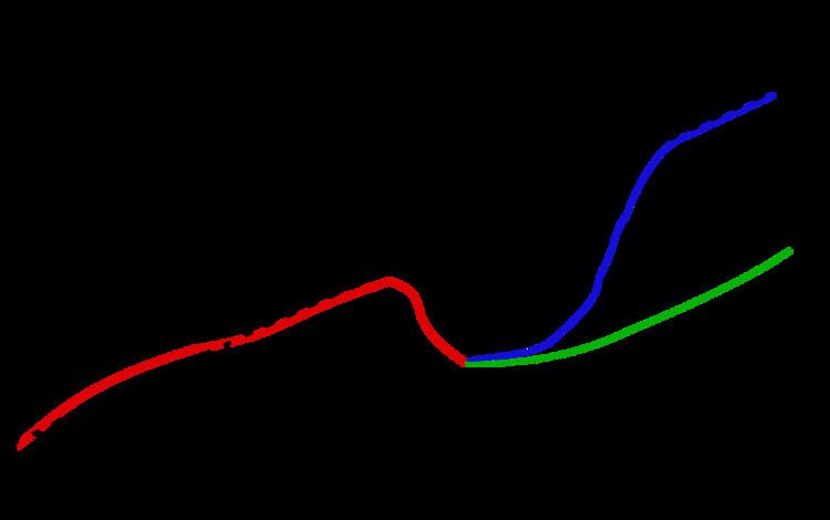
Unit root processes may sometimes be confused with trend-stationary processes; while they share many properties, they are different in many aspects. It is possible for a time series to be non-stationary, have no unit-root yet be trend-stationary. In both unit root and trend-stationary processes, the mean can be growing or decreasing over time; however, in the presence of a shock, trend-stationary processes are mean-reverting (i.e. transitory, the time series will converge again towards the growing mean, which was not affected by the shock) while unit-root processes have a permanent impact on the mean (i.e. no convergence over time).

If a root of the process's characteristic equation is larger than 1, then it is called an explosive process, even though such processes are often inaccurately called unit roots processes.

The presence of a unit root can be tested using a unit root test.

Definition

Consider a discrete-time stochastic process { y t , t = 1 , … , ∞ } , and suppose that it can be written as an autoregressive process of order p:

y t = a 1 y t − 1 + a 2 y t − 2 + ⋯ + a p y t − p + ε t .

Here, { ε t , t = 0 , ∞ } is a serially uncorrelated, zero-mean stochastic process with constant variance σ 2 . For convenience, assume y 0 = 0 . If m = 1 is a root of the characteristic equation:

m p − m p − 1 a 1 − m p − 2 a 2 − ⋯ − a p = 0

then the stochastic process has a unit root or, alternatively, is integrated of order one, denoted I ( 1 ) . If m = 1 is a root of multiplicity r, then the stochastic process is integrated of order r, denoted I(r).

Example

The first order autoregressive model, y t = a 1 y t − 1 + ε t , has a unit root when a 1 = 1 . In this example, the characteristic equation is m − a 1 = 0 . The root of the equation is m = 1 .

If the process has a unit root, then it is a non-stationary time series. That is, the moments of the stochastic process depend on t . To illustrate the effect of a unit root, we can consider the first order case, starting from y₀ = 0:

y t = y t − 1 + ε t .

By repeated substitution, we can write y t = y 0 + ∑ j = 1 t ε j . Then the variance of y t is given by:

Var ⁡ ( y t ) = ∑ j = 1 t σ 2 = t σ 2 .

The variance depends on t since Var ⁡ ( y 1 ) = σ 2 , while Var ⁡ ( y 2 ) = 2 σ 2 . Note that the variance of the series is diverging to infinity with t.

There are various tests to check for the existence of a unit root, some of them are given by:

The Dickey-Fuller test
Testing the significance of more than one coefficients (f-test)
The Phillips Peron Test (PP) unit root test
Dickey Pantula test

In addition to AR and ARMA models, other important models arise in regression analysis where the model errors may themselves have a time series structure and thus may need to be modelled by an AR or ARMA process that may have a unit root, as discussed above. The finite sample properties of regression models with first order ARMA errors, including unit roots, have been analyzed.

Estimation when a unit root may be present

Often, ordinary least squares (OLS) is used to estimate the slope coefficients of the autoregressive model. Use of OLS relies on the stochastic process being stationary. When the stochastic process is non-stationary, the use of OLS can produce invalid estimates. Granger and Newbold called such estimates 'spurious regression' results: high R² values and high t-ratios yielding results with no economic meaning.

To estimate the slope coefficients, one should first conduct a unit root test, whose null hypothesis is that a unit root is present. If that hypothesis is rejected, one can use OLS. However, if the presence of a unit root is not rejected, then one should apply the difference operator to the series. If another unit root test shows the differenced time series to be stationary, OLS can then be applied to this series to estimate the slope coefficients.

For example, in the AR(1) case, Δ y t = y t − y t − 1 = ε t is stationary.

In the AR(2) case, y t = a 1 y t − 1 + a 2 y t − 2 + ε t can be written as ( 1 − λ 1 L ) ( 1 − λ 2 L ) y t = ε t where L is a lag operator that decreases the time index of a variable by one period: L y t = y t − 1 . If λ 2 = 1 , the model has a unit root and we can define z t = Δ y t ; then

z t = λ 1 z t − 1 + ε t

is stationary if | λ 1 | < 1 . OLS can be used to estimate the slope coefficient, λ 1 .

If the process has multiple unit roots, the difference operator can be applied multiple times.

Properties and characteristics of unit-root processes

Shocks to a unit root process have permanent effects which do not decay as they would if the process were stationary

As noted above, a unit root process has a variance that depends on t, and diverges to infinity

If it is known that a series has a unit root, the series can be differenced to render it stationary. For example, if a series Y t is I(1), the series Δ Y t = Y t − Y t − 1 is I(0) (stationary). It is hence called a difference stationary series.

Unit root hypothesis

Economists debate whether various economic statistics, especially output, have a unit root or are trend stationary. A unit root process with drift is given in the first-order case by

y t = y t − 1 + c + e t

where c is a constant term referred to as the "drift" term, and e t is white noise. Any non-zero value of the noise term, occurring for only one period, will permanently affect the value of y t as shown in the graph, so deviations from the line y t = a + c t are non-stationary; there is no reversion to any trend line. In contrast, a trend stationary process is given by

y t = k ⋅ t + u t

where k is the slope of the trend and u t is noise (white noise in the simplest case; more generally, noise following its own stationary autoregressive process). Here any transient noise will not alter the long-run tendency for y t to be on the trend line, as also shown in the graph. This process is said to be trend stationary because deviations from the trend line are stationary.

The issue is particularly popular in the literature on business cycles. Research on the subject began with Nelson and Plosser whose paper on GNP and other output aggregates failed to reject the unit root hypothesis for these series. Since then, a debate—entwined with technical disputes on statistical methods—has ensued. Some economists argue that GDP has a unit root or structural break, implying that economic downturns result in permanently lower GDP levels in the long run. Other economists argue that GDP is trend-stationary: That is, when GDP dips below trend during a downturn it later returns to the level implied by the trend so that there is no permanent decrease in output. While the literature on the unit root hypothesis may consist of arcane debate on statistical methods, the hypothesis carries significant practical implications for economic forecasts and policies.

References

Unit root Wikipedia

(Text) CC BY-SA

Contents