Autoregressive model

Definition

The notation A R ( p ) indicates an autoregressive model of order p. The AR(p) model is defined as

X t = c + ∑ i = 1 p φ i X t − i + ε t

where φ 1 , … , φ p are the parameters of the model, c is a constant, and ε t is white noise. This can be equivalently written using the backshift operator B as

X t = c + ∑ i = 1 p φ i B i X t + ε t

so that, moving the summation term to the left side and using polynomial notation, we have

ϕ ( B ) X t = c + ε t .

An autoregressive model can thus be viewed as the output of an all-pole infinite impulse response filter whose input is white noise.

Some parameter constraints are necessary for the model to remain wide-sense stationary. For example, processes in the AR(1) model with | φ 1 | ≥ 1 are not stationary. More generally, for an AR(p) model to be wide-sense stationary, the roots of the polynomial z p − ∑ i = 1 p φ i z p − i must lie within the unit circle, i.e., each root z i must satisfy | z i | < 1 .

Intertemporal effect of shocks

In an AR process, a one-time shock affects values of the evolving variable infinitely far into the future. For example, consider the AR(1) model X t = c + φ 1 X t − 1 + ε t . A non-zero value for ε t at say time t=1 affects X 1 by the amount ε 1 . Then by the AR equation for X 2 in terms of X 1 , this affects X 2 by the amount φ 1 ε 1 . Then by the AR equation for X 3 in terms of X 2 , this affects X 3 by the amount φ 1 2 ε 1 . Continuing this process shows that the effect of ε 1 never ends, although if the process is stationary then the effect diminishes toward zero in the limit.

Because each shock affects X values infinitely far into the future from when they occur, any given value X_t is affected by shocks occurring infinitely far into the past. This can also be seen by rewriting the autoregression

ϕ ( B ) X t = ε t

(where the constant term has been suppressed by assuming that the variable has been measured as deviations from its mean) as

X t = 1 ϕ ( B ) ε t .

When the polynomial division on the right side is carried out, the polynomial in the backshift operator applied to ε t has an infinite order—that is, an infinite number of lagged values of ε t appear on the right side of the equation.

Characteristic polynomial

The autocorrelation function of an AR(p) process can be expressed as

ρ ( τ ) = ∑ k = 1 p a k y k − | τ | ,

where y k are the roots of the polynomial

ϕ ( B ) = 1 − ∑ k = 1 p φ k B k

where B is the backshift operator, where ϕ ( ⋅ ) is the function defining the autoregression, and where φ k are the coefficients in the autoregression.

The autocorrelation function of an AR(p) process is a sum of decaying exponentials.

Each real root contributes a component to the autocorrelation function that decays exponentially.

Similarly, each pair of complex conjugate roots contributes an exponentially damped oscillation.

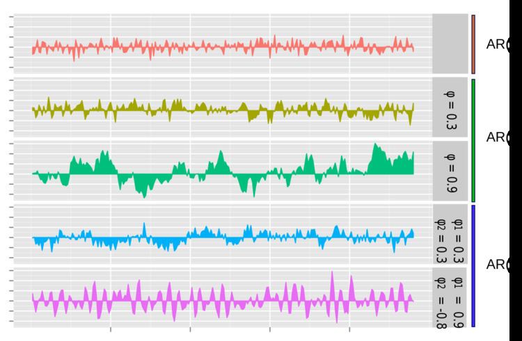
Graphs of AR(p) processes

The simplest AR process is AR(0), which has no dependence between the terms. Only the error/innovation/noise term contributes to the output of the process, so in the figure, AR(0) corresponds to white noise.

For an AR(1) process with a positive φ , only the previous term in the process and the noise term contribute to the output. If φ is close to 0, then the process still looks like white noise, but as φ approaches 1, the output gets a larger contribution from the previous term relative to the noise. This results in a "smoothing" or integration of the output, similar to a low pass filter.

For an AR(2) process, the previous two terms and the noise term contribute to the output. If both φ 1 and φ 2 are positive, the output will resemble a low pass filter, with the high frequency part of the noise decreased. If φ 1 is positive while φ 2 is negative, then the process favors changes in sign between terms of the process. The output oscillates. This can be likened to edge detection or detection of change in direction.

Example: An AR(1) process

An AR(1) process is given by:

X t = c + φ X t − 1 + ε t

where ε t is a white noise process with zero mean and constant variance σ ε 2 . (Note: The subscript on φ 1 has been dropped.) The process is wide-sense stationary if | φ | < 1 since it is obtained as the output of a stable filter whose input is white noise. (If φ = 1 then X t has infinite variance, and is therefore not wide sense stationary.) Assuming | φ | < 1 , the mean E ⁡ ( X t ) is identical for all values of t by the very definition of wide sense stationarity. If the mean is denoted by μ , it follows from

E ⁡ ( X t ) = E ⁡ ( c ) + φ E ⁡ ( X t − 1 ) + E ⁡ ( ε t ) ,

that

μ = c + φ μ + 0 ,

and hence

μ = c 1 − φ .

In particular, if c = 0 , then the mean is 0.

The variance is

var ( X t ) = E ⁡ ( X t 2 ) − μ 2 = σ ε 2 1 − φ 2 ,

where σ ε is the standard deviation of ε t . This can be shown by noting that

var ( X t ) = φ 2 var ( X t − 1 ) + σ ε 2 ,

and then by noticing that the quantity above is a stable fixed point of this relation.

The autocovariance is given by

B n = E ⁡ ( X t + n X t ) − μ 2 = σ ε 2 1 − φ 2 φ | n | .

It can be seen that the autocovariance function decays with a decay time (also called time constant) of τ = − 1 / ln ⁡ ( φ ) [to see this, write B n = K φ | n | where K is independent of n . Then note that φ | n | = e | n | ln ⁡ φ and match this to the exponential decay law e − n / τ ].

The spectral density function is the Fourier transform of the autocovariance function. In discrete terms this will be the discrete-time Fourier transform:

Φ ( ω ) = 1 2 π ∑ n = − ∞ ∞ B n e − i ω n = 1 2 π ( σ ε 2 1 + φ 2 − 2 φ cos ⁡ ( ω ) ) .

This expression is periodic due to the discrete nature of the X j , which is manifested as the cosine term in the denominator. If we assume that the sampling time ( Δ t = 1 ) is much smaller than the decay time ( τ ), then we can use a continuum approximation to B n :

B ( t ) ≈ σ ε 2 1 − φ 2 φ | t |

which yields a Lorentzian profile for the spectral density:

Φ ( ω ) = 1 2 π σ ε 2 1 − φ 2 γ π ( γ 2 + ω 2 )

where γ = 1 / τ is the angular frequency associated with the decay time τ .

An alternative expression for X t can be derived by first substituting c + φ X t − 2 + ε t − 1 for X t − 1 in the defining equation. Continuing this process N times yields

X t = c ∑ k = 0 N − 1 φ k + φ N X t − N + ∑ k = 0 N − 1 φ k ε t − k .

For N approaching infinity, φ N will approach zero and:

X t = c 1 − φ + ∑ k = 0 ∞ φ k ε t − k .

It is seen that X t is white noise convolved with the φ k kernel plus the constant mean. If the white noise ε t is a Gaussian process then X t is also a Gaussian process. In other cases, the central limit theorem indicates that X t will be approximately normally distributed when φ is close to one.

Explicit mean/difference form of AR(1) process

The AR(1) model is the discrete time analogy of the continuous Ornstein-Uhlenbeck process. It is therefore sometimes useful to understand the properties of the AR(1) model cast in an equivalent form. In this form, the AR(1) model is given by:

X t + 1 = X t + θ ( μ − X t ) + ϵ t + 1 , where | θ | < 1 and μ is the model mean.

By putting this in the form X t + 1 = c + ϕ X t , and then expanding the series for X t + n , one can show that:

E ⁡ ( X t + n | X t ) = μ [ 1 − ( 1 − θ ) n ] + X t ( 1 − θ ) n , and Var ⁡ ( X t + n | X t ) = σ 2 [ 1 − ( 1 − θ ) 2 n ] 1 − ( 1 − θ ) 2 .

Choosing the maximum lag

The partial autocorrelation of an AR(p) process is zero at lag p + 1 and greater, so the appropriate maximum lag is the one beyond which the partial autocorrelations are all zero.

Calculation of the AR parameters

There are many ways to estimate the coefficients, such as the ordinary least squares procedure or method of moments (through Yule–Walker equations).

The AR(p) model is given by the equation

X t = ∑ i = 1 p φ i X t − i + ε t .

It is based on parameters φ i where i = 1, ..., p. There is a direct correspondence between these parameters and the covariance function of the process, and this correspondence can be inverted to determine the parameters from the autocorrelation function (which is itself obtained from the covariances). This is done using the Yule–Walker equations.

Yule–Walker equations

The Yule–Walker equations, named for Udny Yule and Gilbert Walker, are the following set of equations.

γ m = ∑ k = 1 p φ k γ m − k + σ ε 2 δ m , 0 ,

where m = 0, ..., p, yielding p + 1 equations. Here γ m is the autocovariance function of X_t, σ ε is the standard deviation of the input noise process, and δ m , 0 is the Kronecker delta function.

Because the last part of an individual equation is non-zero only if m = 0, the set of equations can be solved by representing the equations for m > 0 in matrix form, thus getting the equation

[ γ 1 γ 2 γ 3 ⋮ γ p ] = [ γ 0 γ − 1 γ − 2 … γ 1 γ 0 γ − 1 … γ 2 γ 1 γ 0 … ⋮ ⋮ ⋮ ⋱ γ p − 1 γ p − 2 γ p − 3 … ] [ φ 1 φ 2 φ 3 ⋮ φ p ]

which can be solved for all { φ m ; m = 1 , 2 , ⋯ , p } . The remaining equation for m = 0 is

γ 0 = ∑ k = 1 p φ k γ − k + σ ε 2 ,

which, once { φ m ; m = 1 , 2 , ⋯ , p } are known, can be solved for σ ε 2 .

An alternative formulation is in terms of the autocorrelation function. The AR parameters are determined by the first p+1 elements ρ ( τ ) of the autocorrelation function. The full autocorrelation function can then be derived by recursively calculating

ρ ( τ ) = ∑ k = 1 p φ k ρ ( k − τ )

Examples for some Low-order AR(p) processes

p=1

γ 1 = φ 1 γ 0

Hence ρ 1 = γ 1 / γ 0 = φ 1

p=2

The Yule–Walker equations for an AR(2) process are

Remember that γ − k = γ k

Using the first equation yields ρ 1 = γ 1 / γ 0 = φ 1 1 − φ 2

Using the recursion formula yields ρ 2 = γ 2 / γ 0 = φ 1 2 − φ 2 2 + φ 2 1 − φ 2

Estimation of AR parameters

The above equations (the Yule–Walker equations) provide several routes to estimating the parameters of an AR(p) model, by replacing the theoretical covariances with estimated values. Some of these variants can be described as follows:

Estimation of autocovariances or autocorrelations. Here each of these terms is estimated separately, using conventional estimates. There are different ways of doing this and the choice between these affects the properties of the estimation scheme. For example, negative estimates of the variance can be produced by some choices.

Formulation as a least squares regression problem in which an ordinary least squares prediction problem is constructed, basing prediction of values of X_t on the p previous values of the same series. This can be thought of as a forward-prediction scheme. The normal equations for this problem can be seen to correspond to an approximation of the matrix form of the Yule–Walker equations in which each appearance of an autocovariance of the same lag is replaced by a slightly different estimate.

Formulation as an extended form of ordinary least squares prediction problem. Here two sets of prediction equations are combined into a single estimation scheme and a single set of normal equations. One set is the set of forward-prediction equations and the other is a corresponding set of backward prediction equations, relating to the backward representation of the AR model:

Here predicted of values of X_t would be based on the p future values of the same series. This way of estimating the AR parameters is due to Burg, and is called the Burg method: Burg and later authors called these particular estimates "maximum entropy estimates", but the reasoning behind this applies to the use of any set of estimated AR parameters. Compared to the estimation scheme using only the forward prediction equations, different estimates of the autocovariances are produced, and the estimates have different stability properties. Burg estimates are particularly associated with maximum entropy spectral estimation.

Other possible approaches to estimation include maximum likelihood estimation. Two distinct variants of maximum likelihood are available: in one (broadly equivalent to the forward prediction least squares scheme) the likelihood function considered is that corresponding to the conditional distribution of later values in the series given the initial p values in the series; in the second, the likelihood function considered is that corresponding to the unconditional joint distribution of all the values in the observed series. Substantial differences in the results of these approaches can occur if the observed series is short, or if the process is close to non-stationarity.

Spectrum

The power spectral density of an AR(p) process with noise variance V a r ( Z t ) = σ Z 2 is

S ( f ) = σ Z 2 | 1 − ∑ k = 1 p φ k e − i 2 π f k | 2 .

AR(0)

For white noise (AR(0))

S ( f ) = σ Z 2 .

AR(1)

For AR(1)

S ( f ) = σ Z 2 | 1 − φ 1 e − 2 π i f | 2 = σ Z 2 1 + φ 1 2 − 2 φ 1 cos ⁡ 2 π f

If φ 1 > 0 there is a single spectral peak at f=0, often referred to as red noise. As φ 1 becomes nearer 1, there is stronger power at low frequencies, i.e. larger time lags. This is then a low-pass filter, when applied to full spectrum light, everything except for the red light will be filtered.

If φ 1 < 0 there is a minimum at f=0, often referred to as blue noise. This similarly acts as a high-pass filter, everything except for blue light will be filtered.

AR(2)

AR(2) processes can be split into three groups depending on the characteristics of their roots:

z 1 , z 2 = 1 2 ( φ 1 ± φ 1 2 + 4 φ 2 )

When φ 1 2 + 4 φ 2 < 0 , the process has a pair of complex-conjugate roots, creating a mid-frequency peak at:

f ∗ = 1 2 π cos − 1 ⁡ ( φ 1 ( φ 2 − 1 ) 4 φ 2 )

Otherwise the process has real roots, and:

When φ 1 > 0 it acts as a low-pass filter on the white noise with a spectral peak at f = 0

When φ 1 < 0 it acts as a high-pass filter on the white noise with a spectral peak at f = 1 / 2 .

The process is non-stationary when the roots are outside the unit circle. The process is stable when the roots are within the unit circle, or equivalently when the coefficients are in the triangle − 1 ≤ φ 2 ≤ 1 − | φ 1 | .

The full PSD function can be expressed in real form as:

S ( f ) = σ Z 2 1 + φ 1 2 + φ 2 2 − 2 φ 1 ( 1 − φ 2 ) cos ⁡ ( 2 π f ) − 2 φ 2 cos ⁡ ( 4 π f )

Implementations in statistics packages

R, the stats package includes an ar function.

MATLAB's Econometrics Toolbox and System Identification Toolbox includes autoregressive models

Matlab and Octave: the TSA toolbox contains several estimation functions for uni-variate, multivariate and adaptive autoregressive models.

Impulse response

The impulse response of a system is the change in an evolving variable in response to a change in the value of a shock term k periods earlier, as a function of k. Since the AR model is a special case of the vector autoregressive model, the computation of the impulse response in Vector autoregression#Impulse response applies here.

n-step-ahead forecasting

Once the parameters of the autoregression

X t = c + ∑ i = 1 p φ i X t − i + ε t

have been estimated, the autoregression can be used to forecast an arbitrary number of periods into the future. First use t to refer to the first period for which data is not yet available; substitute the known prior values X_t-i for i=1, ..., p into the autoregressive equation while setting the error term ε t equal to zero (because we forecast X_t to equal its expected value, and the expected value of the unobserved error term is zero). The output of the autoregressive equation is the forecast for the first unobserved period. Next, use t to refer to the next period for which data is not yet available; again the autoregressive equation is used to make the forecast, with one difference: the value of X one period prior to the one now being forecast is not known, so its expected value—the predicted value arising from the previous forecasting step—is used instead. Then for future periods the same procedure is used, each time using one more forecast value on the right side of the predictive equation until, after p predictions, all p right-side values are predicted values from prior steps.

There are four sources of uncertainty regarding predictions obtained in this manner: (1) uncertainty as to whether the autoregressive model is the correct model; (2) uncertainty about the accuracy of the forecasted values that are used as lagged values in the right side of the autoregressive equation; (3) uncertainty about the true values of the autoregressive coefficients; and (4) uncertainty about the value of the error term ε t for the period being predicted. Each of the last three can be quantified and combined to give a confidence interval for the n-step-ahead predictions; the confidence interval will become wider as n increases because of the use of an increasing number of estimated values for the right-side variables.

Evaluating the quality of forecasts

The predictive performance of the autoregressive model can be assessed as soon as estimation has been done if cross-validation is used. In this approach, some of the initially available data was used for parameter estimation purposes, and some (from available observations later in the data set) was held back for out-of-sample testing. Alternatively, after some time has passed after the parameter estimation was conducted, more data will have become available and predictive performance can be evaluated then using the new data.

In either case, there are two aspects of predictive performance that can be evaluated: one-step-ahead and n-step-ahead performance. For one-step-ahead performance, the estimated parameters are used in the autoregressive equation along with observed values of X for all periods prior to the one being predicted, and the output of the equation is the one-step-ahead forecast; this procedure is used to obtain forecasts for each of the out-of-sample observations. To evaluate the quality of n-step-ahead forecasts, the forecasting procedure in the previous section is employed to obtain the predictions.

Given a set of predicted values and a corresponding set of actual values for X for various time periods, a common evaluation technique is to use the mean squared prediction error; other measures are also available (see Forecasting#Forecasting accuracy).

The question of how to interpret the measured forecasting accuracy arises—for example, what is a "high" (bad) or a "low" (good) value for the mean squared prediction error? There are two possible points of comparison. First, the forecasting accuracy of an alternative model, estimated under different modeling assumptions or different estimation techniques, can be used for comparison purposes. Second, the out-of-sample accuracy measure can be compared to the same measure computed for the in-sample data points (that were used for parameter estimation) for which enough prior data values are available (that is, dropping the first p data points, for which p prior data points are not available). Since the model was estimated specifically to fit the in-sample points as well as possible, it will usually be the case that the out-of-sample predictive performance will be poorer than the in-sample predictive performance. But if the predictive quality deteriorates out-of-sample by "not very much" (which is not precisely definable), then the forecaster may be satisfied with the performance.