 | ||
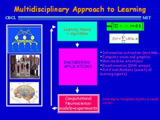
9 520 09 09 2015 class 01 prof tomaso poggio the course at a glance
Statistical learning theory is a framework for machine learning drawing from the fields of statistics and functional analysis. Statistical learning theory deals with the problem of finding a predictive function based on data. Statistical learning theory has led to successful applications in fields such as computer vision, speech recognition, bioinformatics and baseball.
Contents
- 9 520 09 09 2015 class 01 prof tomaso poggio the course at a glance
- An introduction to concentration inequalities and statistical learning theory
- Introduction
- Formal description
- Loss functions
- Regression
- Classification
- Regularization
- References
An introduction to concentration inequalities and statistical learning theory
Introduction
The goals of learning are understanding and prediction. Learning falls into many categories, including supervised learning, unsupervised learning, online learning, and reinforcement learning. From the perspective of statistical learning theory, supervised learning is best understood. Supervised learning involves learning from a training set of data. Every point in the training is an input-output pair, where the input maps to an output. The learning problem consists of inferring the function that maps between the input and the output, such that the learned function can be used to predict output from future input.
Depending on the type of output, supervised learning problems are either problems of regression or problems of classification. If the output takes a continuous range of values, it is a regression problem. Using Ohm's Law as an example, a regression could be performed with voltage as input and current as output. The regression would find the functional relationship between voltage and current to be
Classification problems are those for which the output will be an element from a discrete set of labels. Classification is very common for machine learning applications. In facial recognition, for instance, a picture of a person's face would be the input, and the output label would be that person's name. The input would be represented by a large multidimensional vector whose elements represent pixels in the picture.
After learning a function based on the training set data, that function is validated on a test set of data, data that did not appear in the training set.
Formal description
Take
Every
In this formalism, the inference problem consists of finding a function
The target function, the best possible function
Because the probability distribution
A learning algorithm that chooses the function
Loss functions
The choice of loss function is a determining factor on the function
Different loss functions are used depending on whether the problem is one of regression or one of classification.
Regression
The most common loss function for regression is the square loss function (also known as the L2-norm). This familiar loss function is used in ordinary least squares regression. The form is:
The absolute value loss (also known as the L1-norm) is also sometimes used:
Classification
In some sense the 0-1 indicator function is the most natural loss function for classification. It takes the value 0 if the predicted output is the same as the actual output, and it takes the value 1 if the predicted output is different from the actual output. For binary classification with
where
Regularization
In machine learning problems, a major problem that arises is that of overfitting. Because learning is a prediction problem, the goal is not to find a function that most closely fits the (previously observed) data, but to find one that will most accurately predict output from future input. Empirical risk minimization runs this risk of overfitting: finding a function that matches the data exactly but does not predict future output well.
Overfitting is symptomatic of unstable solutions; a small perturbation in the training set data would cause a large variation in the learned function. It can be shown that if the stability for the solution can be guaranteed, generalization and consistency are guaranteed as well. Regularization can solve the overfitting problem and give the problem stability.
Regularization can be accomplished by restricting the hypothesis space
One example of regularization is Tikhonov regularization. This consists of minimizing
where
