Trisha Shetty (Editor)

Shifted Gompertz distribution

Updated on
Edit
Like
Comment
Share on FacebookTweet on TwitterShare on LinkedInShare on Reddit
Shifted Gompertz distribution

Parameters
  
b ≥ 0 {\displaystyle b\geq 0} scale (real) η ≥ 0 {\displaystyle \eta \geq 0} shape (real)

Support
  
x ∈ [ 0 , ∞ ) {\displaystyle x\in [0,\infty )\!}

PDF
  
b e − b x e − η e − b x [ 1 + η ( 1 − e − b x ) ] {\displaystyle be^{-bx}e^{-\eta e^{-bx}}\left[1+\eta \left(1-e^{-bx}\right)\right]}

CDF
  
( 1 − e − b x ) e − η e − b x {\displaystyle \left(1-e^{-bx}\right)e^{-\eta e^{-bx}}}

Mean
  
( − 1 / b ) { E [ ln ⁡ ( X ) ] − ln ⁡ ( η ) } {\displaystyle (-1/b)\{\mathrm {E} [\ln(X)]-\ln(\eta )\}\,} where X = η e − b x {\displaystyle X=\eta e^{-bx}\,} and E [ ln ⁡ ( X ) ] = [ 1 + 1 / η ] ∫ 0 η e − X [ ln ⁡ ( X ) ] d X − 1 / η ∫ 0 η X e − X [ ln ⁡ ( X ) ] d X {\displaystyle {\begin{aligned}\mathrm {E} [\ln(X)]=&[1{+}1/\eta ]\!\!\int _{0}^{\eta }\!\!\!\!e^{-X}[\ln(X)]dX\\&-1/\eta \!\!\int _{0}^{\eta }\!\!\!\!Xe^{-X}[\ln(X)]dX\end{aligned}}}

Mode
  
0  for  0 < η ≤ 0.5 {\displaystyle 0{\text{ for }}0<\eta \leq 0.5} ( − 1 / b ) ln ⁡ ( z ⋆ ) , for  η > 0.5 {\displaystyle (-1/b)\ln(z^{\star }){\text{, for }}\eta >0.5}  where  z ⋆ = [ 3 + η − ( η 2 + 2 η + 5 ) 1 / 2 ] / ( 2 η ) {\displaystyle {\text{ where }}z^{\star }=[3+\eta -(\eta ^{2}+2\eta +5)^{1/2}]/(2\eta )}

The shifted Gompertz distribution is the distribution of the largest of two independent random variables one of which has an exponential distribution with parameter b and the other has a Gumbel distribution with parameters η and b . In its original formulation the distribution was expressed referring to the Gompertz distribution instead of the Gumbel distribution but, since the Gompertz distribution is a reverted Gumbel distribution, the labelling can be considered as accurate. It has been used as a model of adoption of innovations. It was proposed by Bemmaor (1994). Some of its statistical properties have been studied further by Jiménez and Jodrá (2009) and Jiménez Torres (2014).

Contents

It has been used to predict the growth and decline of social networks and on-line services and shown to be superior to the Bass model and Weibull distribution (Bauckhage and Kersting 2014).

Probability density function

The probability density function of the shifted Gompertz distribution is:

f ( x ; b , η ) = b e b x e η e b x [ 1 + η ( 1 e b x ) ]  for  x 0.

where b 0 is a scale parameter and η 0 is a shape parameter. In the context of diffusion of innovations, b can be interpreted as the overall appeal of the innovation and η is the propensity to adopt in the propensity-to-adopt paradigm. The larger b is, the stronger the appeal and the larger η is, the smaller the propensity to adopt.

The distribution can be reparametrized according to the innovation-imitation paradigm with p = f ( 0 ; b , η ) = b e η as the coefficient of innovation and q = b p as the coefficient of imitation. Hence:

f ( x ; p , q ) = ( p + q ) e ( p + q ) x e ln ( 1 + q / p ) e ( p + q ) x [ 1 + ln ( 1 + q / p ) ( 1 e ( p + q ) x ) ]  for  x 0 , p , q 0. = ( p + q ) e ( p + q ) x ( 1 + q / p ) e ( p + q ) x [ 1 + ln ( 1 + q / p ) ( 1 e ( p + q ) x ) ]  for  x 0 , p , q 0.

When q = 0 , the shifted Gompertz distribution reduces to an exponential distribution. When p = 0 , the proportion of adopters is nill: the innovation is a complete failure. The shape parameter becomes equal to q / p .

Cumulative distribution function

The cumulative distribution function of the shifted Gompertz distribution is:

F ( x ; b , η ) = ( 1 e b x ) e η e b x  for  x 0.

Equivalently,

F ( x ; p , q ) = ( 1 e ( p + q ) x ) e ln ( 1 + q / p ) e ( p + q ) x  for  x 0. = ( 1 e ( p + q ) x ) ( 1 + q / p ) e ( p + q ) x  for  x 0.

Properties

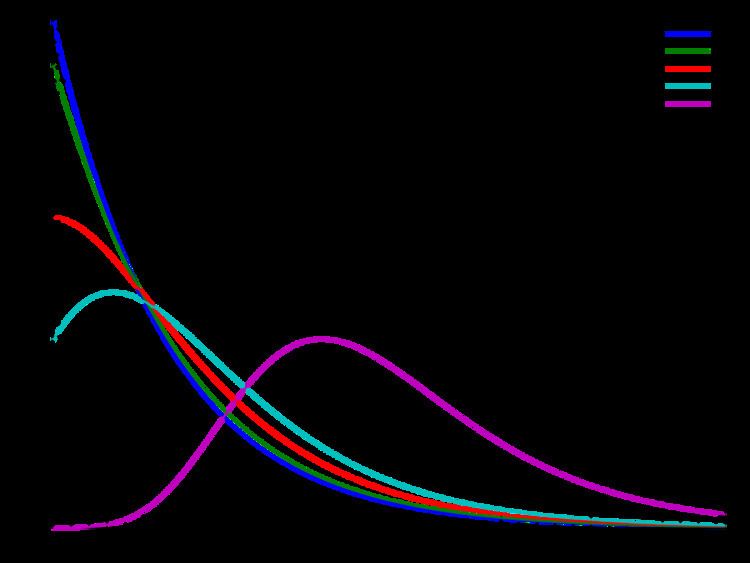
The shifted Gompertz distribution is right-skewed for all values of η . It is more flexible than the Gumbel distribution. The hazard function is a concave function of F ( x ; b , η ) which increases from b e η to b : its curvature is all the steeper as η is large. Contrary to some other distributions, the hazard function cannot be expressed as a closed-form expression of F ( x ; b , η ) . In the context of the diffusion of innovations, the effect of word of mouth on the likelihood to adopt is stronger at the early stages of adoption than at the later ones. The parameter q = b ( 1 e η ) captures the growth of the hazard function from t = 0 to .

Shapes

The shifted Gompertz density function can take on different shapes depending on the values of the shape parameter η :

  • 0 < η 0.5 the probability density function has its mode at 0.
  • η > 0.5 the probability density function has its mode at
  • where z is the smallest root of η 2 z 2 η ( 3 + η ) z + η + 1 = 0 , which is

    When η varies according to a gamma distribution with shape parameter α and scale parameter β (mean = α β ), the distribution of x is Gamma/Shifted Gompertz (G/SG). When α is equal to one, the G/SG reduces to the Bass model (Bemmaor 1994). The three-parameter G/SG has been applied by Dover, Goldenberg and Shapira (2009) and Van den Bulte and Stremersch (2004) among others in the context of the diffusion of innovations. The model is discussed in Chandrasekaran and Tellis (2007).Similar to the shifted Gompertz distribution, the G/SG can either be represented according to the propensity-to-adopt paradigm or according to the innovation-imitation paradigm. In the latter case, it includes three parameters: p , q and α with p = f ( 0 ; b , β , α ) = b / ( 1 + β ) α and q = b p . The parameter α modifies the curvature of the hazard rate as expressed as a function of F ( x ; p , q , α ) : it is convex when α is less than one, linear when α is equal to one, and concave when α is larger than one. Similar to the shifted Gompertz distribution, there is no closed-form expression of the hazard function except when α = 1 . Here are some special cases of the G/SG distribution in its innovation-imitation formulation:

    F ( x ; p , q , α = 0 ) = Exponential ( p + q ) F ( x ; p , q , α = 1 / 2 ) = Competing two-parameter distribution ( p , q ) F ( x ; p , q , α = 1 ) = Bass model ( p , q ) F ( x ; p , q , α = ) = Shifted Gompertz ( p , q )

    with:

    F ( x ; p , q , α = 1 / 2 ) = ( 1 e ( p + q ) x ) / ( 1 + ( q / p ) ( 2 + q / p ) e ( p + q ) x ) 1 / 2  for  x 0 , p , q 0.

    One can compare the parameters p and q across the values of α as they capture the same notions. In all the cases, the hazard function is either constant or a monotonically increasing function of F ( x ; p , q , α ) (positive word of mouth). As the diffusion curve is all the more skewed as α becomes large, we expect q to decrease as the level of skew increases.

    References

    Shifted Gompertz distribution Wikipedia