In the theory of renewal processes, a part of the mathematical theory of probability, the residual time or the forward recurrence time is the time between any given time t and the next epoch of the renewal process under consideration. In the context of random walks, it is also known as overshoot.
The residual time is very important in most of the practical applications of renewal processes:
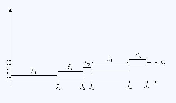
In queueing theory, it determines the remaining time, that a newly arriving customer to a non-empty queue has to wait until being served.In wireless networking, it determines, for example, the remaining lifetime of a wireless link on arrival of a new packet.In dependability studies, it models the remaining lifetime of a component.etc.Consider a renewal process { N ( t ) , t ≥ 0 } , with holding times S i and jump times (or renewal epochs) J i , and i ∈ N . The holding times S i are non-negative, independent, identically distributed random variables and the renewal process is defined as N ( t ) = sup { n : J n ≤ t } . Then, to a given time t , there corresponds uniquely an N ( t ) , such that:
J N ( t ) ≤ t < J N ( t ) + 1 . The residual time (or excess time) is given by the time Y ( t ) from t to the next renewal epoch.
Y ( t ) = J N ( t ) + 1 − t . Let the cumulative distribution function of the holding times S i be F ( t ) = P r [ S i ≤ t ] and recall that the renewal function of a process is m ( t ) = E [ N ( t ) ] . Then, for a given time t , the cumulative distribution function of Y ( t ) is calculated as:
Φ ( x , t ) = Pr [ Y ( t ) ≤ x ] = F ( t + x ) − ∫ 0 t [ 1 − F ( t + x − y ) ] d m ( y ) Differentiating with respect to x , the probability density function can be written as
ϕ ( x , t ) = f ( t + x ) + ∫ 0 t f ( u + x ) m ′ ( t − u ) d u From elementary renewal theorem m ′ ( t ) → 1 / μ as t → ∞ . If we consider the limiting distribution as t → ∞ , assuming that f ( t ) → 0 as t → ∞ , we have the limiting pdf as
ϕ ( x ) = 1 μ ∫ 0 ∞ f ( u + x ) d u = 1 μ ∫ x ∞ f ( v ) d v = 1 − F ( x ) μ , where μ is the mean of the distribution F . Likewise, the cumulative distribution of the residual time is
Φ ( x ) = 1 μ ∫ 0 x [ 1 − F ( x ) ] d u . For large t , the distribution is independent of t , making it a stationary distribution. An interesting fact is that the limiting distribution of forward recurrence time (or residual time) has the same form as the limiting distribution of the backward recurrence time (or age). This distribution is always J-shaped, with mode at zero.
When the holding times S i are exponentially distributed with F ( t ) = 1 − e − λ t , the residual times are also exponentially distributed. That is because m ( t ) = λ t and:
Pr [ Y ( t ) ≤ x ] = [ 1 − e − λ ( t + x ) ] − ∫ 0 t [ 1 − 1 + e − λ ( t + x − y ) ] d ( λ y ) = 1 − e − λ x . This is a known characteristic of the exponential distribution, i.e., its memoryless property. Intuitively, this means that it does not matter how long it has been since the last renewal epoch, the remaining time is still probabilistically the same as in the beginning of the holding time interval.
Renewal theory texts usually also define the spent time or the backward recurrence time (or the current lifetime) as Z ( t ) = t − J N ( t ) . Its distribution can be calculated in a similar way to that of the residual time. However, the spent time has much less practical interest than the residual time.