Iterative reconstruction

Basic concepts

The reconstruction of an image from the acquired data is an inverse problem. Often, it is not possible to exactly solve the inverse problem directly. In this case, a direct algorithm has to approximate the solution, which might cause visible reconstruction artifacts in the image. Iterative algorithms approach the correct solution using multiple iteration steps, which allows to obtain a better reconstruction at the cost of a higher computation time.

In computed tomography, this approach was the one first used by Hounsfield. There are a large variety of algorithms, but each starts with an assumed image, computes projections from the image, compares the original projection data and updates the image based upon the difference between the calculated and the actual projections.

There are typically five components to iterative image reconstruction algorithms, e.g. .

1. An object model that expresses the unknown continuous-space function f ( r ) that is to be reconstructed in terms of a finite series with unknown coefficients that must be estimated from the data.
2. A system model that relates the unknown object to the "ideal" measurements that would be recorded in the absence of measurement noise. Often this is a linear model of the form A x + ϵ , where ϵ represents the noise.
3. A statistical model that describes how the noisy measurements vary around their ideal values. Often Gaussian noise or Poisson statistics are assumed. Because Poisson statistics are closer to reality, it is more widely used.
4. A cost function that is to be minimized to estimate the image coefficient vector. Often this cost function includes some form of regularization. Sometimes the regularization is based on Markov random fields.
5. An algorithm, usually iterative, for minimizing the cost function, including some initial estimate of the image and some stopping criterion for terminating the iterations.

Advantages

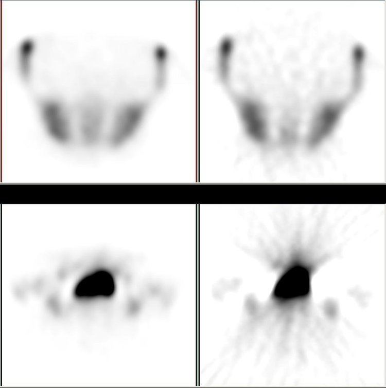
The advantages of the iterative approach include improved insensitivity to noise and capability of reconstructing an optimal image in the case of incomplete data. The method has been applied in emission tomography modalities like SPECT and PET, where there is significant attenuation along ray paths and noise statistics are relatively poor.

Statistical, likelihood-based approaches: Statistical, likelihood-based iterative expectation-maximization algorithms are now the preferred method of reconstruction. Such algorithms compute estimates of the likely distribution of annihilation events that led to the measured data, based on statistical principle, often providing better noise profiles and resistance to the streak artifacts common with FBP. Since the density of radioactive tracer is a function in a function space, therefore of extremely high-dimensions, methods which regularize the maximum-likelihood solution turning it towards penalized or maximum a-posteriori methods can have significant advantages for low counts. Examples such as Ulf Grenander's Sieve estimator or Bayes penalty methods or via I.J. Good's roughness method , may yield superior performance to expectation-maximization-based methods which involve a Poisson likelihood function only.

As another example, it is considered superior when one does not have a large set of projections available, when the projections are not distributed uniformly in angle, or when the projections are sparse or missing at certain orientations. These scenarios may occur in intraoperative CT, in cardiac CT, or when metal artifacts require the exclusion of some portions of the projection data.

In Magnetic Resonance Imaging it can be used to reconstruct images from data acquired with multiple receive coils and with sampling patterns different from the conventional Cartesian grid and allows the use of improved regularization techniques (e.g. total variation) or an extended modeling of physical processes to improve the reconstruction. For example, with iterative algorithms it is possible to reconstruct images from data acquired in a very short time as required for Real-time MRI.

In Cryo Electron Tomography, where the limited number of projections are acquired due to the hardware limitations and to avoid the biological specimen damage, it can be used along with compressive sensing techniques or regularization functions (e.g. Huber function) to improve the reconstruction for better interpretation.

Here is an example that illustrates the benefits of iterative image reconstruction for cardiac MRI.