Objective stress rate - Alchetron, The Free Social Encyclopedia

In continuum mechanics, objective stress rates are time derivatives of stress that do not depend on the frame of reference. Many constitutive equations are designed in the form of a relation between a stress-rate and a strain-rate (or the rate of deformation tensor). The mechanical response of a material should not depend on the frame of reference. In other words, material constitutive equations should be frame indifferent (objective). If the stress and strain measures are material quantities then objectivity is automatically satisfied. However, if the quantities are spatial, then the objectivity of the stress-rate is not guaranteed even if the strain-rate is objective.

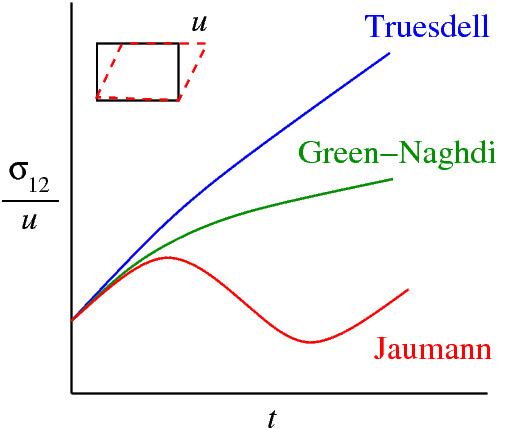
The adjacent figure shows the performance of various objective rates in a simple shear test where the material model is hypoelastic with constant elastic moduli. The ratio of the shear stress to the displacement is plotted as a function of time. The same moduli are used with the three objective stress rates. Clearly there are spurious oscillations observed for the Jaumann stress rate. This is not because one rate is better than another but because it is a misuse of material models to use the same constants with different objective rates. For this reason, a recent trend has been to avoid objective stress rates altogether where possible.

Non-objectivity of the time derivative of Cauchy stress

Under rigid body rotations ( Q ), the Cauchy stress tensor σ transforms as

σ r = Q ⋅ σ ⋅ Q T ; Q ⋅ Q T = 1

Since σ is a spatial quantity and the transformation follows the rules of tensor transformations, σ is objective. However,

d d t ( σ r ) = σ ˙ r = Q ˙ ⋅ σ ⋅ Q T + Q ⋅ σ ˙ ⋅ Q T + Q ⋅ σ ⋅ Q ˙ T ≠ Q ⋅ σ ˙ ⋅ Q T .

Therefore, the stress rate is not objective unless the rate of rotation is zero, i.e. Q is constant.

For a physical understanding of the above, consider the situation shown in Figure 1. In the figure the components of the Cauchy (or true) stress tensor are denoted by the symbols S i j . This tensor, which describes the forces on a small material element imagined to be cut out from the material as currently deformed, is not objective at large deformations because it varies with rigid body rotations of the material. The material points must be characterized by their initial Lagrangian coordinates X i . Consequently, it is necessary to introduce the so-called objective stress rate S ∘ i j , or the corresponding increment Δ S i j = S ∘ i j Δ t . The objectivity is necessary for S ∘ i j to be functionally related to the element deformation. It means that S ∘ i j must be invariant with respect to coordinate transformations, particularly the rigid-body rotations, and must characterize the state of the same material element as it deforms.

The objective stress rate can be derived in two ways:

by tensorial coordinate transformations, which is the standard way in finite element textbooks

variationally, from strain energy density in the material expressed in terms of the strain tensor (which is objective by definition)

While the former way is instructive and provides useful geometric insight, the latter way is mathematically shorter and has the additional advantage of automatically ensuring energy conservation, i.e., guaranteeing that the second-order work of the stress increment tensor on the strain increment tensor be correct (work conjugacy requirement).

Truesdell stress rate of the Cauchy stress

The relation between the Cauchy stress and the 2nd P-K stress is called the Piola transformation. This transformation can be written in terms of the pull-back of σ or the push-forward of S as

S = J ϕ ∗ [ σ ] ; σ = J − 1 ϕ ∗ [ S ]

The Truesdell rate of the Cauchy stress is the Piola transformation of the material time derivative of the 2nd P-K stress. We thus define

σ ∘ = J − 1 ϕ ∗ [ S ˙ ]

Expanded out, this means that

σ ∘ = J − 1 F ⋅ S ˙ ⋅ F T = J − 1 F ⋅ [ d d t ( J F − 1 ⋅ σ ⋅ F − T ) ] ⋅ F T = J − 1 L φ [ τ ]

where the Kirchhoff stress τ = J σ and the Lie derivative of the Kirchhoff stress is

L φ [ τ ] = F ⋅ [ d d t ( F − 1 ⋅ τ ⋅ F − T ) ] ⋅ F T .

This expression can be simplified to the well known expression for the Truesdell rate of the Cauchy stress

It can be shown that the Truesdell rate is objective.

Truesdell rate of the Kirchhoff stress

The Truesdell rate of the Kirchhoff stress can be obtained by noting that

S = ϕ ∗ [ τ ] ; τ = ϕ ∗ [ S ]

and defining

τ ∘ = ϕ ∗ [ S ˙ ]

Expanded out, this means that

τ ∘ = F ⋅ S ˙ ⋅ F T = F ⋅ [ d d t ( F − 1 ⋅ τ ⋅ F − T ) ] ⋅ F T = L φ [ τ ]

Therefore, the Lie derivative of τ is the same as the Truesdell rate of the Kirchhoff stress.

Following the same process as for the Cauchy stress above, we can show that

Green-Naghdi rate of the Cauchy stress

This is a special form of the Lie derivative (or the Truesdell rate of the Cauchy stress). Recall that the Truesdell rate of the Cauchy stress is given by

σ ∘ = J − 1 F ⋅ [ d d t ( J F − 1 ⋅ σ ⋅ F − T ) ] ⋅ F T .

From the polar decomposition theorem we have

F = R ⋅ U

where R is the orthogonal rotation tensor ( R − 1 = R T ) and U is the symmetric, positive definite, right stretch.

If we assume that U = 1 we get F = R . Also since there is no stretch J = 1 and we have τ = σ . Note that this doesn't mean that there is not stretch in the actual body - this simplification is just for the purposes of defining an objective stress rate. Therefore,

σ ∘ = R ⋅ [ d d t ( R − 1 ⋅ σ ⋅ R − T ) ] ⋅ R T = R ⋅ [ d d t ( R T ⋅ σ ⋅ R ) ] ⋅ R T

We can show that this expression can be simplified to the commonly used form of the Green-Naghdi rate

The Green–Naghdi rate of the Kirchhoff stress also has the form since the stretch is not taken into consideration, i.e.,

τ ◻ = τ ˙ + τ ⋅ Ω − Ω ⋅ τ

Jaumann rate of the Cauchy stress

The Jaumann rate of the Cauchy stress is a further specialization of the Lie derivative (Truesdell rate). This rate has the form

The Jaumann rate is used widely in computations primarily for two reasons

it is relatively easy to implement.
it leads to symmetric tangent moduli.

Recall that the spin tensor w (the skew part of the velocity gradient) can be expressed as

w = R ˙ ⋅ R T + 1 2 R ⋅ ( U ˙ ⋅ U − 1 − U − 1 ⋅ U ˙ ) ⋅ R T

Thus for pure rigid body motion

w = R ˙ ⋅ R T = Ω

Alternatively, we can consider the case of proportional loading when the principal directions of strain remain constant. An example of this situation is the axial loading of a cylindrical bar. In that situation, since

U = [ λ X λ Y λ Z ]

we have

U ˙ = [ λ ˙ X λ ˙ Y λ ˙ Z ]

Also,

U − 1 = [ 1 / λ X 1 / λ Y 1 / λ Z ] of the Cauchy stress

Therefore,

U ˙ ⋅ U − 1 = [ λ ˙ X / λ X λ ˙ Y / λ Y λ ˙ Z / λ Z ] = U − 1 U ˙

This once again gives

w = R ˙ ⋅ R T = Ω

In general, if we approximate

w ≈ R ˙ ⋅ R T

the Green–Naghdi rate becomes the Jaumann rate of the Cauchy stress

σ △ = σ ˙ + σ ⋅ w − w ⋅ σ

Other objective stress rates

There can be an infinite variety of objective stress rates. One of these is the Oldroyd stress rate

σ ▽ = L φ [ σ ] = F ⋅ [ d d t ( F − 1 ⋅ σ ⋅ F − T ) ] ⋅ F T

In simpler form, the Oldroyd rate is given by

σ ▽ = σ ˙ − l ⋅ σ − σ ⋅ l T

If the current configuration is assumed to be the reference configuration then the pull back and push forward operations can be conducted using F T and F − T respectively. The Lie derivative of the Cauchy stress is then called the convective stress rate

σ ⋄ = F − T ⋅ [ d d t ( F T ⋅ σ ⋅ F ) ] ⋅ F − 1

In simpler form, the convective rate is given by

σ ⋄ = σ ˙ + l ⋅ σ + σ ⋅ l T

Objective stress rates in finite strain inelasticity

Many materials undergo inelastic deformations caused by plasticity and damage. These material behaviors cannot be described in terms of a potential. It is also often the case that no memory of the initial virgin state exists, particularly when large deformations are involved. The constitutive relation is typically defined in incremental form in such cases to make the computation of stresses and deformations easier.

The incremental loading procedure

For a small enough load step, the material deformation can be characterized by the small (or linearized) strain increment tensor

e = 1 2 [ ∇ u + ( ∇ u ) T ] ≡ e i j = 1 2 ( u i , j + u j , i )

where u is the displacement increment of the continuum points. The time derivative

∂ e ∂ t = e ˙ = 1 2 [ ∇ v + ( ∇ v ) T ] ≡ e ˙ i j = 1 2 ( v i , j + v j , i )

is the strain rate tensor (also called the velocity strain) and v = u ˙ is the material point velocity or displacement rate. For finite strains, measures from the Seth–Hill family (also called Doyle–Ericksen tensors) can be used:

E ( m ) = 1 2 m ( U 2 m − I )

where U is the right stretch. A second-order approximation of these tensors is

E ( m ) ≈ e + 1 2 ( ∇ u ) T ⋅ ∇ u − ( 1 − m ) e ⋅ e

Energy-consistent objective stress rates

Consider a material element of unit initial volume, starting from an initial state under initial Cauchy (or true) stress σ 0 and let σ be the Cauchy stress in the final configuration. Let W be the work done (per unit initial volume) by the internal forces during an incremental deformation from this initial state. Then the variation δ W corresponds to the variation in the work done due to a variation in the displacement δ u . The displacement variation has to satisfy the displacement boundary conditions.

Let S ( m ) be an objective stress tensor in the initial configuration. Define the stress increment with respect to the initial configuration is S = S ( m ) − σ 0 . Alternatively, if P is the unsymmetric first Piola–Kirchhoff stress referred to the initial configuration, the increment in stress can be expressed as T = P − σ 0 .

Variation of work done

Then the variation in work done can be expressed as

δ W = S ( m ) : δ E ( m ) = P : δ ∇ u

where the finite strain measure E ( m ) is energy conjugate to the stress measure σ ( m ) . Expanded out,

δ W = ( S + σ 0 ) : δ E ( m ) = ( T + σ 0 ) : δ ∇ u .

The objectivity of stress tensor S ( m ) is ensured by its transformation as a second-order tensor under coordinate rotations (which causes the principal stresses to be independent from coordinate rotations) and by the correctness of S ( m ) : δ E ( m ) as a second-order energy expression.

From the symmetry of the Cauchy stress, we have

σ 0 : δ ∇ u = σ 0 : δ e .

For small variations in strain, using the approximation

S : δ E ( m ) ≈ S : δ ∇ u

and the expansions

σ 0 : δ E ( m ) = σ 0 : [ ∂ E ( m ) ∂ ∇ u : δ ∇ u ] , σ 0 : δ e = σ 0 : [ ∂ e ∂ ∇ u : δ ∇ u ]

we get the equation

σ 0 : [ ∂ E ( m ) ∂ ∇ u : δ ∇ u ] + S : δ ∇ u = σ 0 : [ ∂ e ∂ ∇ u : δ ∇ u ] + T : δ ∇ u .

Imposing the variational condition that the resulting equation must be valid for any strain gradient δ ∇ u , we have

( 1 ) S = T − σ 0 : [ ∂ E ( m ) ∂ ∇ u − ∂ e ∂ ∇ u ]

We can also write the above equation as

( 2 ) S ( m ) = P − σ 0 : ∂ ∂ ∇ u [ E ( m ) − e ] .

Time derivatives

The Cauchy stress and the first Piola-Kirchhoff stress are related by (see Stress measures)

σ = P ⋅ F T J − 1 = ( P + P ⋅ ∇ u T ) J − 1 .

For small incremental deformations,

J − 1 ≈ 1 − ∇ ⋅ u .

Therefore,

Δ σ = σ − σ 0 ≈ ( P + P ⋅ ∇ u T ) ( 1 − ∇ ⋅ u ) − σ 0 .

Substituting T + σ 0 = P ,

Δ σ ≈ [ T + σ 0 + ( T + σ 0 ) ⋅ ∇ u T ] ( 1 − ∇ ⋅ u ) − σ 0 .

For small increments of stress T relative to the initial stress σ 0 , the above reduces to

( 3 ) Δ σ ≈ T − σ 0 ( ∇ ⋅ u ) + σ 0 ⋅ ∇ u T .

From equations (1) and (3) we have

( 4 ) S = Δ σ + σ 0 ( ∇ ⋅ u ) − σ 0 ⋅ ∇ u T − σ 0 : [ ∂ E ( m ) ∂ ∇ u − ∂ e ∂ ∇ u ]

Recall that S is an increment of the stress tensor measure S ( m ) . Defining the stress rate

S =: S ∘ ( m ) Δ t

and noting that

Δ σ = σ ˙ Δ t

we can write equation (4) as

( 5 ) S ∘ ( m ) Δ t = σ ˙ Δ t + σ 0 ( ∇ ⋅ v ) Δ t − σ 0 ⋅ ∇ v T Δ t − σ 0 : [ ∂ E ( m ) ∂ ∇ u − ∂ e ∂ ∇ u ]

Taking the limit at Δ t → 0 , and noting that σ 0 = σ at this limit, one gets the following expression for the objective stress rate associated with the strain measure E ( m ) :

( 6 ) S ∘ ( m ) = σ ˙ + σ ( ∇ ⋅ v ) − σ ⋅ ∇ v T − σ : ∂ ∂ t [ ∂ ∂ ∇ u ( E ( m ) − e ) ] .

Here σ ˙ i j = ∂ σ i j / ∂ t = material rate of Cauchy stress (i.e., the rate in Lagrangian coordinates of the initial stressed state).

Work-conjugate stress rates

A rate for which there exists no legitimate finite strain tensor E ( m ) associated according to Eq. (6) is energetically inconsistent, i.e., its use violates energy balance (i.e., the first law of thermodynamics).

Evaluating Eq. (6) for general m and for m = 2 , one gets a general expression for the objective stress rate:

( 7 ) S ∘ ( m ) = S ∘ ( 2 ) + 1 2 ( 2 − m ) [ σ ⋅ e ˙ + ( σ ⋅ e ˙ ) T ]

where S ∘ ( 2 ) is the objective stress rate associated with the Green-Lagrangian strain ( m = 2 ).

In particular,

m = 2 gives the Truesdell stress rate

m = 0 gives the Jaumann rate of Kirchhoff stress

m = 1 gives the Biot stress rate

(Note that m = 2 leads to Engesser's formula for critical load in shear buckling, while m = -2 leads to Haringx's formula which can give critical loads differing by >100%).

Non work-conjugate stress rates

Other rates, used in most commercial codes, which are not work-conjugate to any finite strain tensor are:

the Jaumann, or corotational, rate of Cauchy stress: It differs from Jaumann rate of Kirchhoff stress by missing the rate of relative volume change of material. The lack of work-conjugacy is usually not a serious problem since that term is negligibly small for many materials and zero for incompressible materials (but in indentation of a sandwich plate with foam core, this rate can give an error of >30% in the indentation force).

the Cotter–Rivlin rate corresponds to m = − 2 but it again misses the volumetric term.

the Green–Naghdi rate: This objective stress rate is not work-conjugate to any finite strain tensor, not only because of missing the volumetric term but also because the material rotation velocity is not exactly equal to the spin tensor. In vast majority of applications, the energy errors caused by these differences are totally negligible but it must be pointed out that a large energy error was already demonstrated for a case with shear strains and rotations exceeding about 0.25.

the Oldroyd rate.

Objective rates and Lie derivatives

The objective stress rates could also be regarded as the Lie derivatives of various types of stress tensor (i.e., the associated covariant, contravariant and mixed components of Cauchy stress) and their linear combinations. The Lie derivative does not include the concept of work-conjugacy.

Tangential stiffness moduli and their transformations to achieve energy consistency

The tangential stress-strain relation has generally the form

( 6 ) S ˙ i j ( m ) = C i j k l ( m ) e ˙ k l

where C i j k l ( m ) are the tangential moduli (components of a 4th-order tensor) associated with strain tensor ϵ i j ( m ) . They are different for different choices of m , and are related as follows:

( 7 ) [ C i j k l ( m ) − C i j k l ( 2 ) − 1 4 ( 2 − m ) ( S i k δ j l + S j k δ i l + S i l δ j k + S j l δ i k ) ] v k , l = 0

From the fact that Eq. (7) must hold true for any velocity gradient v k , l , it follows that:

( 8 ) C i j k l ( m ) = C i j k l ( 2 ) + ( 2 − m ) [ S i k δ j l ] s y m , [ S i k δ j l ] s y m = 1 4 ( S i k δ j l + S j k δ i l + S i l δ j k + S j l δ i k )

where C i j k l ( 2 ) are the tangential moduli associated with the Green–Lagrangian strain ( m = 2 ), taken as a reference, S i j = current Cauchy stress, and δ i j = Kronecker delta (or unit tensor).

Eq. (8) can be used to convert one objective stress rate to another. Since S i j e ˙ k k = ( S i j δ k l ) δ e k l , the transformation

( 9 ) C i j k l c o n j = C i j k l n o n c o n j + S i j δ k l

can further correct for the absence of the term S i j v k , k (note that the term S i j δ k m does not allow interchanging subscripts i j with k l , which means that its absence breaks the major symmetry of the tangential moduli tensor C i j k l n o n c o n j ).

Large strain often develops when the material behavior becomes nonlinear, due to plasticity or damage. Then the primary cause of stress dependence of the tangential moduli is the physical behavior of material. What Eq. (8) means that the nonlinear dependence of C i j k l on the stress must be different for different objective stress rates. Yet none of them is fundamentally preferable, except if there exists one stress rate, one m , for which the moduli can be considered constant.

References

Objective stress rate Wikipedia

(Text) CC BY-SA

Contents