In continuum mechanics, a Mooney–Rivlin solid is a hyperelastic material model where the strain energy density function W is a linear combination of two invariants of the left Cauchy–Green deformation tensor B . The model was proposed by Melvin Mooney in 1940 and expressed in terms of invariants by Ronald Rivlin in 1948.
The strain energy density function for an incompressible Mooney–Rivlin material is
W = C 1 ( I ¯ 1 − 3 ) + C 2 ( I ¯ 2 − 3 ) , where C 1 and C 2 are empirically determined material constants, and I 1 and I 2 are the first and the second invariant of the unimodular component of the left Cauchy–Green deformation tensor:
I ¯ 1 = J − 2 / 3 I 1 ; I 1 = λ 1 2 + λ 2 2 + λ 3 2 ; J = det ( F ) = λ 1 λ 2 λ 3 I ¯ 2 = J − 4 / 3 I 2 ; I 2 = λ 1 2 λ 2 2 + λ 2 2 λ 3 2 + λ 3 2 λ 1 2 where F is the deformation gradient. For an incompressible material, J = 1 .
The Mooney–Rivlin model is a special case of the generalized Rivlin model (also called polynomial hyperelastic model) which has the form
W = ∑ p , q = 0 N C p q ( I ¯ 1 − 3 ) p ( I ¯ 2 − 3 ) q + ∑ m = 1 M D m ( J − 1 ) 2 m with C 00 = 0 where C p q are material constants related to the distortional response and D m are material constants related to the volumetric response. For a compressible Mooney–Rivlin material N = 1 , C 01 = C 2 , C 11 = 0 , C 10 = C 1 , M = 1 and we have
W = C 01 ( I ¯ 2 − 3 ) + C 10 ( I ¯ 1 − 3 ) + D 1 ( J − 1 ) 2 If C 01 = 0 we obtain a neo-Hookean solid, a special case of a Mooney–Rivlin solid.
For consistency with linear elasticity in the limit of small strains, it is necessary that
κ = 2 ⋅ D 1 ; μ = 2 ( C 01 + C 10 ) where κ is the bulk modulus and μ is the shear modulus.
The Cauchy stress in a compressible hyperelastic material with a stress free reference configuration is given by
σ = 2 J [ 1 J 2 / 3 ( ∂ W ∂ I ¯ 1 + I ¯ 1 ∂ W ∂ I ¯ 2 ) B − 1 J 4 / 3 ∂ W ∂ I ¯ 2 B ⋅ B ] + [ ∂ W ∂ J − 2 3 J ( I ¯ 1 ∂ W ∂ I ¯ 1 + 2 I ¯ 2 ∂ W ∂ I ¯ 2 ) ] 1 For a compressible Mooney–Rivlin material,
∂ W ∂ I ¯ 1 = C 1 ; ∂ W ∂ I ¯ 2 = C 2 ; ∂ W ∂ J = 2 D 1 ( J − 1 ) Therefore, the Cauchy stress in a compressible Mooney–Rivlin material is given by
σ = 2 J [ 1 J 2 / 3 ( C 1 + I ¯ 1 C 2 ) B − 1 J 4 / 3 C 2 B ⋅ B ] + [ 2 D 1 ( J − 1 ) − 2 3 J ( C 1 I ¯ 1 + 2 C 2 I ¯ 2 ) ] 1 It can be shown, after some algebra, that the pressure is given by
p := − 1 3 tr ( σ ) = − ∂ W ∂ J = − 2 D 1 ( J − 1 ) . The stress can then be expressed in the form
σ = 1 J [ − p 1 + 2 J 2 / 3 ( C 1 + I ¯ 1 C 2 ) B − 2 J 4 / 3 C 2 B ⋅ B − 2 3 ( C 1 I ¯ 1 + 2 C 2 I ¯ 2 ) 1 ] . The above equation is often written as
σ = 1 J [ − p 1 + 2 ( C 1 + I ¯ 1 C 2 ) B ¯ − 2 C 2 B ¯ ⋅ B ¯ − 2 3 ( C 1 I ¯ 1 + 2 C 2 I ¯ 2 ) 1 ] where B ¯ = J − 2 / 3 B . For an incompressible Mooney–Rivlin material with J = 1
σ = 2 ( C 1 + I ¯ 1 C 2 ) B − 2 C 2 B ⋅ B − 2 3 ( C 1 I ¯ 1 + 2 C 2 I ¯ 2 ) 1 . Note that if J = 1 then
det ( B ) = det ( F ) det ( F T ) = 1 Then, from the Cayley-Hamilton theorem,
B − 1 = B ⋅ B − I 1 B + I 2 1 Hence, the Cauchy stress can be expressed as
σ = − p ∗ 1 + 2 C 1 B − 2 C 2 B − 1 where p ∗ := 2 3 ( C 1 I 1 − C 2 I 2 ) .
In terms of the principal stretches, the Cauchy stress differences for an incompressible hyperelastic material are given by
σ 11 − σ 33 = λ 1 ∂ W ∂ λ 1 − λ 3 ∂ W ∂ λ 3 ; σ 22 − σ 33 = λ 2 ∂ W ∂ λ 2 − λ 3 ∂ W ∂ λ 3 For an incompressible Mooney-Rivlin material,
W = C 1 ( λ 1 2 + λ 2 2 + λ 3 2 − 3 ) + C 2 ( λ 1 2 λ 2 2 + λ 2 2 λ 3 2 + λ 3 2 λ 1 2 − 3 ) ; λ 1 λ 2 λ 3 = 1 Therefore,
λ 1 ∂ W ∂ λ 1 = 2 C 1 λ 1 2 + 2 C 2 λ 1 2 ( λ 2 2 + λ 3 2 ) ; λ 2 ∂ W ∂ λ 2 = 2 C 1 λ 2 2 + 2 C 2 λ 2 2 ( λ 1 2 + λ 3 2 ) ; λ 3 ∂ W ∂ λ 3 = 2 C 1 λ 3 2 + 2 C 2 λ 3 2 ( λ 1 2 + λ 2 2 ) Since λ 1 λ 2 λ 3 = 1 . we can write
λ 1 ∂ W ∂ λ 1 = 2 C 1 λ 1 2 + 2 C 2 ( 1 λ 3 2 + 1 λ 2 2 ) ; λ 2 ∂ W ∂ λ 2 = 2 C 1 λ 2 2 + 2 C 2 ( 1 λ 3 2 + 1 λ 1 2 ) λ 3 ∂ W ∂ λ 3 = 2 C 1 λ 3 2 + 2 C 2 ( 1 λ 2 2 + 1 λ 1 2 ) Then the expressions for the Cauchy stress differences become
σ 11 − σ 33 = 2 C 1 ( λ 1 2 − λ 3 2 ) − 2 C 2 ( 1 λ 1 2 − 1 λ 3 2 ) ; σ 22 − σ 33 = 2 C 1 ( λ 2 2 − λ 3 2 ) − 2 C 2 ( 1 λ 2 2 − 1 λ 3 2 ) For the case of an incompressible Mooney–Rivlin material under uniaxial elongation, λ 1 = λ and λ 2 = λ 3 = 1 / λ . Then the true stress (Cauchy stress) differences can be calculated as:
σ 11 − σ 33 = 2 C 1 ( λ 2 − 1 λ ) − 2 C 2 ( 1 λ 2 − λ ) σ 22 − σ 33 = 0 In the case of simple tension, σ 22 = σ 33 = 0 . Then we can write
σ 11 = ( 2 C 1 + 2 C 2 λ ) ( λ 2 − 1 λ ) In alternative notation, where the Cauchy stress is written as T and the stretch as α , we can write
T 11 = ( 2 C 1 + 2 C 2 α ) ( α 2 − α − 1 ) and the engineering stress (force per unit reference area) for an incompressible Mooney–Rivlin material under simple tension can be calculated using T 11 e n g = T 11 α 2 α 3 = T 11 α . Hence
T 11 e n g = ( 2 C 1 + 2 C 2 α ) ( α − α − 2 ) If we define
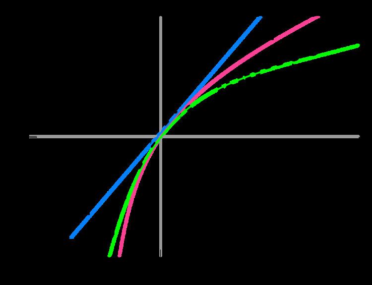
T 11 ∗ := T 11 e n g α − α − 2 ; β := 1 α then
T 11 ∗ = 2 C 1 + 2 C 2 β . The slope of the T 11 ∗ versus β line gives the value of C 2 while the intercept with the T 11 ∗ axis gives the value of C 1 . The Mooney–Rivlin solid model usually fits experimental data better than Neo-Hookean solid does, but requires an additional empirical constant.
In the case of equibiaxial tension, the principal stretches are λ 1 = λ 2 = λ . If, in addition, the material is incompressible then λ 3 = 1 / λ 2 . The Cauchy stress differences may therefore be expressed as
σ 11 − σ 33 = σ 22 − σ 33 = 2 C 1 ( λ 2 − 1 λ 4 ) − 2 C 2 ( 1 λ 2 − λ 4 ) The equations for equibiaxial tension are equivalent to those governing uniaxial compression.
A pure shear deformation can be achieved by applying stretches of the form
λ 1 = λ ; λ 2 = 1 λ ; λ 3 = 1 The Cauchy stress differences for pure shear may therefore be expressed as
σ 11 − σ 33 = 2 C 1 ( λ 2 − 1 ) − 2 C 2 ( 1 λ 2 − 1 ) ; σ 22 − σ 33 = 2 C 1 ( 1 λ 2 − 1 ) − 2 C 2 ( λ 2 − 1 ) Therefore
σ 11 − σ 22 = 2 ( C 1 + C 2 ) ( λ 2 − 1 λ 2 ) For a pure shear deformation
I 1 = λ 1 2 + λ 2 2 + λ 3 2 = λ 2 + 1 λ 2 + 1 ; I 2 = 1 λ 1 2 + 1 λ 2 2 + 1 λ 3 2 = 1 λ 2 + λ 2 + 1 Therefore I 1 = I 2 .
The deformation gradient for a simple shear deformation has the form
F = 1 + γ e 1 ⊗ e 2 where e 1 , e 2 are reference orthonormal basis vectors in the plane of deformation and the shear deformation is given by
γ = λ − 1 λ ; λ 1 = λ ; λ 2 = 1 λ ; λ 3 = 1 In matrix form, the deformation gradient and the left Cauchy-Green deformation tensor may then be expressed as
F = [ 1 γ 0 0 1 0 0 0 1 ] ; B = F ⋅ F T = [ 1 + γ 2 γ 0 γ 1 0 0 0 1 ] Therefore,
B − 1 = [ 1 − γ 0 − γ 1 + γ 2 0 0 0 1 ] The Cauchy stress is given by
σ = [ − p ∗ + 2 ( C 1 − C 2 ) + 2 C 1 γ 2 2 ( C 1 + C 2 ) γ 0 2 ( C 1 + C 2 ) γ − p ∗ + 2 ( C 1 − C 2 ) − 2 C 2 γ 2 0 0 0 − p ∗ + 2 ( C 1 − C 2 ) ] For consistency with linear elasticity, clearly μ = 2 ( C 1 + C 2 ) where μ is the shear modulus.
Elastic response of rubber-like materials are often modeled based on the Mooney—Rivlin model. The constants C 1 , C 2 are determined by fitting the predicted stress from the above equations to the experimental data. The recommended tests are uniaxial tension, equibiaxial compression, equibiaxial tension, uniaxial compression, and for shear, planar tension and planar compression. The two parameter Mooney–Rivlin model is usually valid for strains less than 100%.