
 | ||
A neo-Hookean solid is a hyperelastic material model, similar to Hooke's law, that can be used for predicting the nonlinear stress-strain behavior of materials undergoing large deformations. The model was proposed by Ronald Rivlin in 1948. In contrast to linear elastic materials, the stress-strain curve of a neo-Hookean material is not linear. Instead, the relationship between applied stress and strain is initially linear, but at a certain point the stress-strain curve will plateau. The neo-Hookean model does not account for the dissipative release of energy as heat while straining the material and perfect elasticity is assumed at all stages of deformation.
Contents
- Compressible neo Hookean material
- Incompressible neo Hookean material
- Pure dilation
- Simple shear
- References
The neo-Hookean model is based on the statistical thermodynamics of cross-linked polymer chains and is usable for plastics and rubber-like substances. Cross-linked polymers will act in a neo-Hookean manner because initially the polymer chains can move relative to each other when a stress is applied. However, at a certain point the polymer chains will be stretched to the maximum point that the covalent cross links will allow, and this will cause a dramatic increase in the elastic modulus of the material. The neo-Hookean material model does not predict that increase in modulus at large strains and is typically accurate only for strains less than 20%. The model is also inadequate for biaxial states of stress and has been superseded by the Mooney-Rivlin model.
The strain energy density function for an incompressible neo-Hookean material in a three-dimensional description is
where
where
where
where, in this case,
Several alternative formulations exist for compressible neo-Hookean materials, for example
For consistency with linear elasticity,
where
Compressible neo-Hookean material
For a compressible Rivlin neo-Hookean material the Cauchy stress is given by
where
For infinitesimal strains (
and the Cauchy stress can be expressed as
Comparison with Hooke's law shows that
Incompressible neo-Hookean material
For an incompressible neo-Hookean material with
where
Compressible neo-Hookean material
For a compressible neo-Hookean hyperelastic material, the principal components of the Cauchy stress are given by
Therefore, the differences between the principal stresses are
Incompressible neo-Hookean material
In terms of the principal stretches, the Cauchy stress differences for an incompressible hyperelastic material are given by
For an incompressible neo-Hookean material,
Therefore,
which gives
Compressible neo-Hookean material
For a compressible material undergoing uniaxial extension, the principal stretches are
Hence, the true (Cauchy) stresses for a compressible neo-Hookean material are given by
The stress differences are given by
If the material is unconstrained we have
Equating the two expressions for
or
The above equation can be solved numerically using a Newton-Raphson iterative root finding procedure.
Incompressible neo-Hookean material
Under uniaxial extension,
Assuming no traction on the sides,
where
The equation above is for the true stress (ratio of the elongation force to deformed cross-section). For the engineering stress the equation is:
For small deformations
Thus, the equivalent Young's modulus of a neo-Hookean solid in uniaxial extension is
Compressible neo-Hookean material
In the case of equibiaxial extension
Therefore,
The stress differences are
If the material is in a state of plane stress then
We also have a relation between
or,
This equation can be solved for
Incompressible neo-Hookean material
For an incompressible material
Under plane stress conditions we have
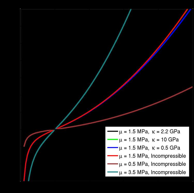
Pure dilation
For the case of pure dilation
Therefore, the principal Cauchy stresses for a compressible neo-Hookean material are given by
If the material is incompressible then
The figures below show that extremely high stresses are needed to achieve large triaxial extensions or compressions. Equivalently, relatively small triaxial stretch states can cause very high stresses to develop in a rubber-like material. Note also that the magnitude of the stress is quite sensitive to the bulk modulus but not to the shear modulus.
Simple shear
For the case of simple shear the deformation gradient in terms of components with respect to a reference basis is of the form
where
Compressible neo-Hookean material
In this case
Hence the Cauchy stress is given by
Incompressible neo-Hookean material
Using the relation for the Cauchy stress for an incompressible neo-Hookean material we get
Thus neo-Hookean solid shows linear dependence of shear stresses upon shear deformation and quadratic dependence of the normal stress difference on the shear deformation. Note that the expressions for the Cauchy stress for a compressible and an incompressible neo-Hookean material in simple shear represent the same quantity and provide a means of determining the unknown pressure