
 | ||
In the mathematical subfield of numerical analysis, monotone cubic interpolation is a variant of cubic interpolation that preserves monotonicity of the data set being interpolated.
Contents
- Monotone cubic Hermite interpolation
- Interpolant selection
- Cubic interpolation
- Example implementation
- References
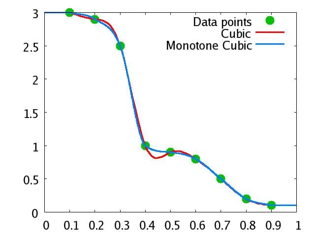
Monotonicity is preserved by linear interpolation but not guaranteed by cubic interpolation.
Monotone cubic Hermite interpolation
Monotone interpolation can be accomplished using cubic Hermite spline with the tangents
An algorithm is also available for monotone quintic Hermite interpolation.
Interpolant selection
There are several ways of selecting interpolating tangents for each data point. This section will outline the use of the Fritsch–Carlson method.
Let the data points be
- Compute the slopes of the secant lines between successive points:
forΔ k = y k + 1 − y k x k + 1 − x k k = 1 , … , n − 1 . - Initialize the tangents at every data point as the average of the secants,
form k = Δ k − 1 + Δ k 2 k = 2 , … , n − 1 ; ifΔ k − 1 Δ k m k = 0 . These may be updated in further steps. For the endpoints, use one-sided differences:m 1 = Δ 1 and m n = Δ n − 1 - For
k = 1 , … , n − 1 , ifΔ k = 0 (if two successivey k = y k + 1 m k = m k + 1 = 0 , as the spline connecting these points must be flat to preserve monotonicity. Ignore step 4 and 5 for thosek . - Let
α k = m k / Δ k β k = m k + 1 / Δ k α k β k − 1 ( x k , y k ) is a local extremum. In such cases, piecewise monotone curves can still be generated by choosingm k = 0 , although global strict monotonicity is not possible. - To prevent overshoot and ensure monotonicity, at least one of the following conditions must be met:
- the function
must have a value greater than or equal to zero;ϕ ( α , β ) = α − ( 2 α + β − 3 ) 2 3 ( α + β − 2 ) -
α + 2 β − 3 ≤ 0 ; or -
2 α + β − 3 ≤ 0 .
- the function
If monotonicity must be strict then
One simple way to satisfy this constraint is to restrict the vector
Alternatively it is sufficient to restrict
Note that only one pass of the algorithm is required.
Cubic interpolation
After the preprocessing, evaluation of the interpolated spline is equivalent to cubic Hermite spline, using the data
To evaluate at
then the interpolant is
where
Example implementation
The following JavaScript implementation takes a data set and produces a monotone cubic spline interpolant function: