
 | ||
In algebra, a quintic function is a function of the form
Contents
- Finding roots of a quintic equation
- Solvable quintics
- Quintics in BringJerrard form
- Roots of a solvable quintic
- Other solvable quintics
- Casus irreducibilis
- Beyond radicals
- Solving through Bring radical
- Application to celestial mechanics
- References
where a, b, c, d, e and f are members of a field, typically the rational numbers, the real numbers or the complex numbers, and a is nonzero. In other words, a quintic function is defined by a polynomial of degree five.
If a is zero but one of the coefficients b, c, d, or e is non-zero, the function is classified as either a quartic function, cubic function, quadratic function or linear function.
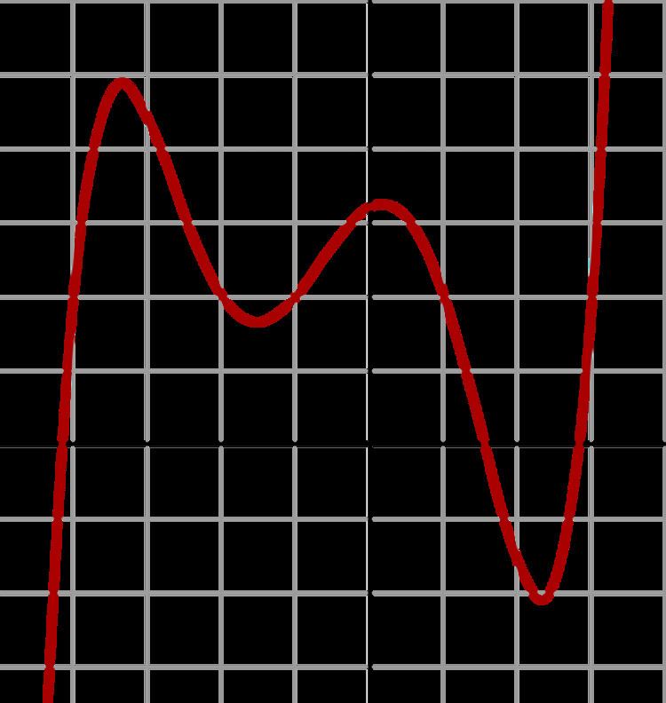
Because they have an odd degree, normal quintic functions appear similar to normal cubic functions when graphed, except they may possess an additional local maximum and local minimum each. The derivative of a quintic function is a quartic function.
Setting g(x) = 0 and assuming a ≠ 0 produces a quintic equation of the form:
Solving quintic equations in terms of radicals was a major problem in algebra, from the 16th century, when cubic and quartic equations were solved, until the first half of the 19th century, when the impossibility of such a general solution was proved, with the Abel–Ruffini theorem.
Finding roots of a quintic equation
Finding the roots of a given polynomial has been a prominent mathematical problem.
Solving linear, quadratic, cubic and quartic equations by factorization into radicals can always be done, no matter whether the roots are rational or irrational, real or complex; there are formulae that yield the required solutions. However, there is no algebraic expression for general quintic equations over the rationals in terms of radicals; this statement is known as the Abel–Ruffini theorem, first published in 1799. This result also holds for equations of higher degrees. An example of a quintic whose roots cannot be expressed in terms of radicals is x5 − x + 1 = 0. This quintic is in Bring–Jerrard normal form.
Some quintics may be solved in terms of radicals. However, the solution is generally too complex to be used in practice. Instead, numerical approximations are calculated using root-finding algorithm for polynomials.
Solvable quintics
Some quintic equations can be solved in terms of radicals. These include the quintic equations defined by a polynomial that is reducible, such as x5 − x4 − x + 1 = (x2 + 1)(x + 1)(x − 1)2. As solving reducible quintic equations reduces immediately to solving polynomials of lower degree, only irreducible quintic equations are considered in this section, and the term "quintic" will refer only to irreducible quintics. A solvable quintic is thus an irreducible quintic polynomial whose roots may be expressed in terms of radicals.
For characterizing solvable quintics, and more generally solvable polynomials of higher degree, Évariste Galois developed techniques which gave rise to group theory and Galois theory. Applying these techniques, Arthur Cayley found a general criterion for determining whether any given quintic is solvable. This criterion is the following.
Given the equation
the Tschirnhaus transformation x = y − b/5a, which depresses the quintic (that means removes the term of degree four), gives the equation
where
Both quintics are solvable by radicals if and only if either they are factorisable in equations of lower degrees with rational coefficients or the polynomial P2 − 1024zΔ, named Cayley's resolvent, has a rational root in z, where
and
Cayley's result allows us to test if a quintic is solvable. If it is the case, finding its roots is a more difficult problem, which consists of expressing the roots in terms of radicals involving the coefficients of the quintic and the rational root of Cayley's resolvent.
In 1888, George Paxton Young described how to solve a solvable quintic equation, without providing an explicit formula; Daniel Lazard wrote out a three-page formula (Lazard (2004)).
Quintics in Bring–Jerrard form
There are several parametric representations of solvable quintics of the form x5 + ax + b = 0, called the Bring–Jerrard form.
During the second half of 19th century, John Stuart Glashan, George Paxton Young, and Carl Runge gave such a parameterization: an irreducible quintic with rational coefficients in Bring–Jerrard form is solvable if and only if either a = 0 or it may be written
where μ and ν are rational.
In 1994, Blair Spearman and Kenneth S. Williams gave an alternative,
The relationship between the 1885 and 1994 parameterizations can be seen by defining the expression
where a = 5(4ν + 3)/ν2 + 1. Using the negative case of the square root yields, after scaling variables, the first parametrization while the positive case gives the second.
The substitution c = −m/l5, e = 1/l in the Spearman-Williams parameterization allows one to not exclude the special case a = 0, giving the following result:
If a and b are rational numbers, the equation x5 + ax + b = 0 is solvable by radicals if either its left-hand side is a product of polynomials of degree less than 5 with rational coefficients or there exist two rational numbers l and m such that
Roots of a solvable quintic
A polynomial equation is solvable by radicals if its Galois group is a solvable group. In the case of irreducible quintics, the Galois group is a subgroup of the symmetric group S5 of all permutations of a five element set, which is solvable if and only if it is a subgroup of the group F5, of order 20, generated by the cyclic permutations (1 2 3 4 5) and (1 2 4 3).
If the quintic is solvable, one of the solutions may be represented by an algebraic expression involving a fifth root and at most two square roots, generally nested. The other solutions may then obtained either by changing of fifth root or by multiplying all the occurrences of the fifth root by the same power of a primitive 5th root of unity
(The other primitive 5th roots of unity may be deduced by changing the signs of the square roots.)
It follows that one may need four different square roots for writing all the roots of a solvable quintic. Even for the first root that involves at most two square roots, the expression of the solutions in terms of radicals is usually huge. However, when no square root is needed, the form of the first solution may be rather simple, as for the equation x5 − 5x4 + 30x3 − 50x2 + 55x − 21 = 0, for which the only real solution is
An example of a more complex (although small enough to be written here) solution is the unique real root of x5 − 5x + 12 = 0. Let a = √2φ−1, b = √2φ, and c = 4√5, where φ = 1+√5/2 is the golden ratio. Then the only real solution x = −1.84208… is given by
or, equivalently, by
where the yi are the four roots of the quartic equation
More generally, if an equation P(x) = 0 of prime degree p with rational coefficients is solvable in radicals, then one can define an auxiliary equation Q(y) = 0 of degree p – 1, also with rational coefficients, such that each root of P is the sum of p-th roots of the roots of Q. These p-th roots have been introduced by Joseph-Louis Lagrange, and their product by p are commonly called Lagrange resolvents. The computation of Q and its roots can be used to solve P(x) = 0. However these p-th roots may not be computed independently (this would provide pp–1 roots instead of p). Thus a correct solution needs to express all these p-roots in term of one of them. Galois theory shows that this is always theoretically possible, even if the resulting formula may be too large to be of any use.
It is possible that some of the roots of Q are rational (as in the first example of this section) or some are zero. In these cases, the formula for the roots is much simpler, as for the solvable de Moivre quintic
where the auxiliary equation has two zero roots and reduces, by factoring them out, to the quadratic equation
such that the five roots of the de Moivre quintic are given by
where yi is any root of the auxiliary quadratic equation and ω is any of the four primitive 5th roots of unity. This can be easily generalized to construct a solvable septic and other odd degrees, not necessarily prime.
Other solvable quintics
There are infinitely many solvable quintics in Bring-Jerrard form which have been parameterized in a preceding section.
Up to the scaling of the variable, there are exactly five solvable quintics of the shape
Paxton Young (1888) gave a number of examples, some of them being reducible, having a rational root:
An infinite sequence of solvable quintics may be constructed, whose roots are sums of n-th roots of unity, with n = 10k + 1 being a prime number:
There are also two parameterized families of solvable quintics: The Kondo–Brumer quintic,
and the family depending on the parameters
where
Casus irreducibilis
Analogously to cubic equations, there are solvable quintics which have five real roots all of whose solutions in radicals involve roots of complex numbers. This is casus irreducibilis for the quintic, which is discussed in Dummit.
Beyond radicals
About 1835, Jerrard demonstrated that quintics can be solved by using ultraradicals (also known as Bring radicals), the unique real root of t5 + t − a = 0 for real numbers a. In 1858 Charles Hermite showed that the Bring radical could be characterized in terms of the Jacobi theta functions and their associated elliptic modular functions, using an approach similar to the more familiar approach of solving cubic equations by means of trigonometric functions. At around the same time, Leopold Kronecker, using group theory, developed a simpler way of deriving Hermite's result, as had Francesco Brioschi. Later, Felix Klein came up with a method that relates the symmetries of the icosahedron, Galois theory, and the elliptic modular functions that are featured in Hermite's solution, giving an explanation for why they should appear at all, and developed his own solution in terms of generalized hypergeometric functions. Similar phenomena occur in degree 7 (septic equations) and 11, as studied by Klein and discussed in icosahedral symmetry: related geometries.
Solving through Bring radical
A Tschirnhaus transformation, which may be computed by solving a quartic equation, reduces the general quintic equation of the form
to the Bring–Jerrard normal form x5 − x + t = 0.
The roots of this equation cannot be expressed by radicals. However, in 1858, Charles Hermite published the first known solution of this equation in terms of elliptic functions. At around the same time Francesco Brioschi and Leopold Kronecker came upon equivalent solutions.
See Bring radical for details on these solutions and some related ones.
Application to celestial mechanics
Solving for the locations of the Lagrangian points of an astronomical orbit in which the masses of both objects are non-negligible involves solving a quintic.
More precisely, the locations of L2 and L1 are the solutions to the following equations, where the gravitational forces of two masses on a third (e.g. Sun and Earth on satellites such as Gaia at L2 and SOHO at L1) provide the satellite's centripetal force necessary to be in a synchronous orbit with Earth around the Sun:
The ± sign corresponds to L2 and L1, respectively; G is the gravitational constant, ω the angular velocity, r the distance of the satellite to Earth, R the distance Sun to Earth (i.e. the semi-major axis of Earth's orbit), and m, MS, and ME are the respective masses of satellite, Earth, and Sun.
Using Kepler's Third Law
with
Solving these two quintics yields r = 1.501 x 10⁹ m for L2 and r = 1.491 x 10⁹ m for L1. The Sun–Earth Lagrangian points L2 and L1 are usually given as 1.5 million km from Earth.