
 | ||
In mathematical optimization, the method of Lagrange multipliers (named after Joseph Louis Lagrange) is a strategy for finding the local maxima and minima of a function subject to equality constraints.
Contents
- Context and method
- Single constraint
- Multiple constraints
- Modern formulation via differentiable manifolds
- Interpretation of the Lagrange multipliers
- Sufficient conditions
- Example 1
- Example 2
- Example 3 Entropy
- Example 4 Numerical optimization
- Economics
- Control theory
- Nonlinear programming
- References
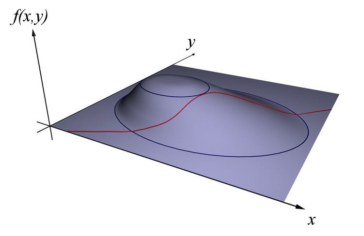
For instance (see Figure 1), consider the optimization problem
maximize f(x, y)subject to g(x, y) = c.We need both f and g to have continuous first partial derivatives. We introduce a new variable (λ) called a Lagrange multiplier and study the Lagrange function (or Lagrangian or Lagrangian expression) defined by
where the λ term may be either added or subtracted. If f(x0, y0) is a maximum of f(x, y) for the original constrained problem, then there exists λ0 such that (x0, y0, λ0) is a stationary point for the Lagrange function (stationary points are those points where the partial derivatives of
Context and method
One of the most common problems in calculus is that of finding maxima or minima (in general, "extrema") of a function, but it is often difficult to find a closed form for the function being extremized. Such difficulties often arise when one wishes to maximize or minimize a function subject to fixed outside equality constraints. The method of Lagrange multipliers is a powerful tool for solving this class of problems without the need to explicitly solve the conditions and use them to eliminate extra variables.
Single constraint
Consider the two-dimensional problem introduced above
maximize f(x, y)subject to g(x, y) = 0.The method of Lagrange multipliers relies on the intuition that at a maximum, f(x, y) cannot be increasing in the direction of any neighboring point where g = 0. If it were, we could walk along g = 0 to get higher, meaning that the starting point wasn't actually the maximum.
We can visualize contours of f given by f(x, y) = d for various values of d, and the contour of g given by g(x, y) = 0.
Suppose we walk along the contour line with g = 0. We are interested in finding points where f does not change as we walk, since these points might be maxima. There are two ways this could happen: First, we could be following a contour line of f, since by definition f does not change as we walk along its contour lines. This would mean that the contour lines of f and g are parallel here. The second possibility is that we have reached a "level" part of f, meaning that f does not change in any direction.
To check the first possibility, notice that since the gradient of a function is perpendicular to the contour lines, the contour lines of f and g are parallel if and only if the gradients of f and g are parallel. Thus we want points (x, y) where g(x, y) = 0 and
for some λ
where
are the respective gradients. The constant λ is required because although the two gradient vectors are parallel, the magnitudes of the gradient vectors are generally not equal. This constant is called the Lagrange multiplier. (In some conventions λ is preceded by a minus sign).
Notice that this method also solves the second possibility: if f is level, then its gradient is zero, and setting λ = 0 is a solution regardless of g.
To incorporate these conditions into one equation, we introduce an auxiliary function
and solve
Note that this amounts to solving three equations in three unknowns. This is the method of Lagrange multipliers. Note that
The method generalizes readily to functions on
which amounts to solving
The constrained extrema of f are critical points of the Lagrangian
One may reformulate the Lagrangian as a Hamiltonian, in which case the solutions are local minima for the Hamiltonian. This is done in optimal control theory, in the form of Pontryagin's minimum principle.
The fact that solutions of the Lagrangian are not necessarily extrema also poses difficulties for numerical optimization. This can be addressed by computing the magnitude of the gradient, as the zeros of the magnitude are necessarily local minima, as illustrated in the numerical optimization example.
Multiple constraints
The method of Lagrange multipliers can be extended to solve problems with multiple constraints using a similar argument. Consider a paraboloid subject to two line constraints that intersect at a single point. As the only feasible solution, this point is obviously a constrained extremum. However, the level set of
Concretely, suppose we have
We are still interested in finding points where
These scalars are the Lagrange multipliers. We now have
As before, we introduce an auxiliary function
and solve
which amounts to solving
The method of Lagrange multipliers is generalized by the Karush–Kuhn–Tucker conditions, which can also take into account inequality constraints of the form h(x) ≤ c.
Modern formulation via differentiable manifolds
Finding local maxima of a function
When
While the above idea sounds good, it is difficult to compute
if and only if
writing
By the first isomorphism theorem this is true if and only if there exists a linear map
in the variables
In the case of several constraints, we work with
Interpretation of the Lagrange multipliers
Often the Lagrange multipliers have an interpretation as some quantity of interest. For example, if the Lagrangian expression is
then
So, λk is the rate of change of the quantity being optimized as a function of the constraint parameter. As examples, in Lagrangian mechanics the equations of motion are derived by finding stationary points of the action, the time integral of the difference between kinetic and potential energy. Thus, the force on a particle due to a scalar potential, F = −∇V, can be interpreted as a Lagrange multiplier determining the change in action (transfer of potential to kinetic energy) following a variation in the particle's constrained trajectory. In control theory this is formulated instead as costate equations.
Moreover, by the envelope theorem the optimal value of a Lagrange multiplier has an interpretation as the marginal effect of the corresponding constraint constant upon the optimal attainable value of the original objective function: if we denote values at the optimum with an asterisk, then it can be shown that
For example, in economics the optimal profit to a player is calculated subject to a constrained space of actions, where a Lagrange multiplier is the change in the optimal value of the objective function (profit) due to the relaxation of a given constraint (e.g. through a change in income); in such a context λ* is the marginal cost of the constraint, and is referred to as the shadow price.
Sufficient conditions
Sufficient conditions for a constrained local maximum or minimum can be stated in terms of a sequence of principal minors (determinants of upper-left-justified sub-matrices) of the bordered Hessian matrix of second derivatives of the Lagrangian expression.
Example 1
Suppose we wish to maximize
Using the method of Lagrange multipliers, we have
hence
Now we can calculate the gradient:
and therefore:
Notice that the last equation is the original constraint.
The first two equations yield
By substituting into the last equation we have:
so
which implies that the stationary points are
Evaluating the objective function f at these points yields
Thus the maximum is
Example 2
Suppose we want to find the maximum values of
with the condition that the x and y coordinates lie on the circle around the origin with radius √3, that is, subject to the constraint
As there is just a single constraint, we will use only one multiplier, say λ.
The constraint g(x, y) is identically zero on the circle of radius √3. So any multiple of g(x, y) may be added to f(x, y) leaving f(x, y) unchanged in the region of interest (on the circle where our original constraint is satisfied). Let
Now we can calculate the gradient:
And therefore:
Notice that (iii) is just the original constraint. (i) implies x = 0 or λ = −y. If x = 0 then
Evaluating the objective at these points, we find that
Therefore, the objective function attains the global maximum (subject to the constraints) at
Note that while
Given any neighborhood of
Example 3: Entropy
Suppose we wish to find the discrete probability distribution on the points
For this to be a probability distribution the sum of the probabilities
We use Lagrange multipliers to find the point of maximum entropy,
which gives a system of n equations,
Carrying out the differentiation of these n equations, we get
This shows that all
we find
Hence, the uniform distribution is the distribution with the greatest entropy, among distributions on n points.
Example 4: Numerical optimization
The critical points of Lagrangians occur at saddle points, rather than at local maxima (or minima). Unfortunately, many numerical optimization techniques, such as hill climbing, gradient descent, some of the quasi-Newton methods, among others, are designed to find local maxima (or minima) and not saddle points. For this reason, one must either modify the formulation to ensure that it's a minimization problem (for example, by extremizing the square of the gradient of the Lagrangian as below), or else use an optimization technique that finds stationary points (such as Newton's method without an extremum seeking line search) and not necessarily extrema.
As a simple example, consider the problem of finding the value of x that minimizes
Using Lagrange multipliers, this problem can be converted into an unconstrained optimization problem:
The two critical points occur at saddle points where x = 1 and x = −1.
In order to solve this problem with a numerical optimization technique, we must first transform this problem such that the critical points occur at local minima. This is done by computing the magnitude of the gradient of the unconstrained optimization problem.
First, we compute the partial derivative of the unconstrained problem with respect to each variable:
If the target function is not easily differentiable, the differential with respect to each variable can be approximated as
where
Next, we compute the magnitude of the gradient, which is the square root of the sum of the squares of the partial derivatives:
(Since magnitude is always non-negative, optimizing over the squared-magnitude is equivalent to optimizing over the magnitude. Thus, the ``square root" may be omitted from these equations with no expected difference in the results of optimization.)
The critical points of h occur at x = 1 and x = −1, just as in
Economics
Constrained optimization plays a central role in economics. For example, the choice problem for a consumer is represented as one of maximizing a utility function subject to a budget constraint. The Lagrange multiplier has an economic interpretation as the shadow price associated with the constraint, in this example the marginal utility of income. Other examples include profit maximization for a firm, along with various macroeconomic applications.
Control theory
In optimal control theory, the Lagrange multipliers are interpreted as costate variables, and Lagrange multipliers are reformulated as the minimization of the Hamiltonian, in Pontryagin's minimum principle.
Nonlinear programming
The Lagrange multiplier method has several generalizations. In nonlinear programming there are several multiplier rules, e.g., the Carathéodory-John Multiplier Rule and the Convex Multiplier Rule, for inequality constraints.