
 | ||
In economics, marginal cost is the change in the opportunity cost that arises when the quantity produced is incremented by one unit, that is, it is the cost of producing one more unit of a good. In general terms, marginal cost at each level of production includes any additional costs required to produce the next unit. For example, if producing additional vehicles requires building a new factory, the marginal cost of the extra vehicles includes the cost of the new factory. In practice, this analysis is segregated into short and long-run cases, so that, over the longest run, all costs become marginal. At each level of production and time period being considered, marginal costs include all costs that vary with the level of production, whereas other costs that do not vary with production are considered fixed.
Contents
- Cost functions and relationship to average cost
- Economies of scale
- Perfectly competitive supply curve
- Decisions taken based on marginal costs
- Relationship to fixed costs
- References
The graph is plotted with Price, Cost and Revenue on the Y-axis and Quantity on the X-axis.
If the good being produced is infinitely divisible, the size of a marginal cost will change with volume; so a non-linear and non-proportional cost function includes the following:
In practice the above definition of marginal cost as the change in total cost as a result of an increase in output of one unit is inconsistent with the differential definition of marginal cost for virtually all non-linear functions. This is as the definition finds the tangent to the total cost curve at the point q which assumes that costs increase at the same rate as they were at q. A new definition may be useful for marginal unit cost (MUC) using the current definition of the change in total cost as a result of an increase of one unit of output defined as: TC(q+1)-TC(q) and re-defining marginal cost to be the change in total as a result of an infinitesimally small increase in q which is consistent with its use in economic literature and can be calculated differentially.
If the cost function is differentiable joining, the marginal cost is the cost of the next unit produced referring to the basic volume.
If the cost function is not differentiable, the marginal cost can be expressed as follows.
A number of other factors can affect marginal cost and its applicability to real world problems. Some of these may be considered market failures. These may include information asymmetries, the presence of negative or positive externalities, transaction costs, price discrimination and others.
Cost functions and relationship to average cost
In the simplest case, the total cost function and its derivative are expressed as follows, where Q represents the production quantity, VC represents variable costs, FC represents fixed costs and TC represents total costs.
Since (by definition) fixed costs do not vary with production quantity, it drops out of the equation when it is differentiated. The important conclusion is that marginal cost is not related to fixed costs. This can be compared with average total cost or ATC, which is the total cost divided by the number of units produced and does include fixed costs.
For discrete calculation without calculus, marginal cost equals the change in total (or variable) cost that comes with each additional unit produced. In contrast, incremental cost is the composition of total cost from the surrogate of contributions, where any increment is determined by the contribution of the cost factors, not necessarily by single units.
For instance, suppose the total cost of making 1 shoe is $30 and the total cost of making 2 shoes is $40. The marginal cost of producing the second shoe is $40 – $30 = $10.
Marginal cost is not the cost of producing the "next" or "last" unit. As Silberberg and Suen note, the cost of the last unit is the same as the cost of the first unit and every other unit. In the short run, increasing production requires using more of the variable input — conventionally assumed to be labor. Adding more labor to a fixed capital stock reduces the marginal product of labor because of the diminishing marginal returns. This reduction in productivity is not limited to the additional labor needed to produce the marginal unit - the productivity of every unit of labor is reduced. Thus the costs of producing the marginal unit of output has two components: the cost associated with producing the marginal unit and the increase in average costs for all units produced due to the “damage” to the entire productive process (∂AC/∂q)q. The first component is the per unit or average cost. The second unit is the small increase in costs due to the law of diminishing marginal returns which increases the costs of all units of sold.
Marginal costs can also be expressed as the cost per unit of labor divided by the marginal product of labor.
Because
where MPL is ratio of increase in the quantity produced per unit increase in labour i.e. ΔQ/ΔL. Therefore,
Economies of scale
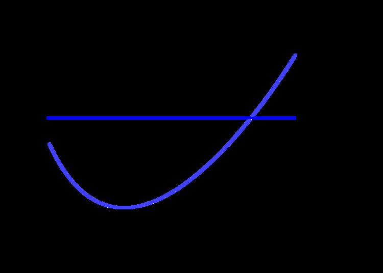
Economies of scale is a concept that applies to the long run, a span of time in which all inputs can be varied by the firm so that there are no fixed inputs or fixed costs. Production may be subject to economies of scale (or diseconomies of scale). Economies of scale are said to exist if an additional unit of output can be produced for less than the average of all previous units— that is, if long-run marginal cost is below long-run average cost, so the latter is falling. Conversely, there may be levels of production where marginal cost is higher than average cost, and average cost is an increasing function of output. For this generic case, minimum average cost occurs at the point where average cost and marginal cost are equal (when plotted, the marginal cost curve intersects the average cost curve from below); this point will not be at the mimum for marginal cost if fixed costs are greater than 0.
Perfectly competitive supply curve
The portion of the marginal cost curve above its intersection with the average variable cost curve is the supply curve for a firm operating in a perfectly competitive market. (the portion of the MC curve below its intersection with the AVC curve is not part of the supply curve because a firm would not operate at price below the shut down point) This is not true for firms operating in other market structures. For example, while a monopoly "has" an MC curve it does not have a supply curve. In a perfectly competitive market, a supply curve shows the quantity a seller's willing and able to supply at each price - for each price there is a unique quantity that would be supplied. The one-to-one relationship simply is absent in the case of a monopoly. With a monopoly there could be an infinite number of prices associated with a given quantity. It all depends on the shape and position of the demand curve and its accompanying marginal revenue curve.
Decisions taken based on marginal costs
In perfectly competitive markets, firms decide the quantity to be produced based on marginal costs and sale price. If the sale price is higher than the marginal cost, then they supply the unit and sell it. If the marginal cost is higher than the price, it would not be profitable to produce it. So the production will be carried out until the marginal cost is equal to the sale price. In other words, firms refuse to sell if the marginal cost is greater than the market price.
Relationship to fixed costs
Marginal costs are not affected by changes in fixed cost. Marginal costs can be expressed as ∆C(q)∕∆Q. Since fixed costs do not vary with (depend on) changes in quantity, MC is ∆VC∕∆Q. Thus if fixed cost were to double, the cost of MC would not be affected, and consequently the profit maximizing quantity and price would not change. This can be illustrated by graphing the short run total cost curve and the short run variable cost curve. The shape of the curves are identical. Each curve initially increases at a decreasing rate, reaches an inflection point, then increases at an increasing rate. The only difference between the curves is that the SRVC curve begins from the origin while the SRTC curve originates on the y-axis. The distance of the origin of the SRTC above the origin represents the fixed cost - the vertical distance between the curves. This distance remains constant as the quantity produced, Q, increases. MC is the slope of the SRVC curve. A change in fixed cost would be reflected by a change in the vertical distance between the SRTC and SRVC curve. Any such change would have no effect on the shape of the SRVC curve and therefore its slope at any point - MC.