LCP array

History

The LCP array was introduced in 1993, by Udi Manber and Gene Myers alongside the suffix array in order to improve the running time of their string search algorithm. Gene Myers later became the vice president of Informatics Research at Celera Genomics, and Udi Manber the vice president of engineering at Google.

Definition

Let A be the suffix array of the string S = s 1 , s 2 , . . . s n $ and let lcp ⁡ ( v , w ) denote the length of the longest common prefix between two strings v and w . Let further denote S [ i , j ] the substring of S ranging from i to j .

Then the LCP array H [ 1 , n ] is an integer array of size n such that H [ 1 ] is undefined and H [ i ] = lcp ⁡ ( S [ A [ i − 1 ] , n ] , S [ A [ i ] , n ] ) for every 1 < i ≤ n . Thus H [ i ] stores the length of longest common prefix of the lexicographically i 'th smallest suffix and its predecessor in the suffix array.

Example

Consider the string S = b a n a n a $ :

and its corresponding sorted suffix array A  :

Complete suffix array with sorted suffixes itself:

Then the LCP array H is constructed by comparing lexicographically consecutive suffixes to determine their longest common prefix:

So, for example, H [ 4 ] = 3 is the length of the longest common prefix a n a shared by the suffixes A [ 3 ] = S [ 4 , 7 ] = a n a $ and A [ 4 ] = S [ 2 , 7 ] = a n a n a $ . Note that H [ 1 ] = ⊥ , since there is no lexicographically smaller suffix.

Difference between suffix array and LCP array

Suffix array: Represents the lexicographic rank of each suffix of an array.

LCP array: Contains the maximum length prefix match between two consecutive suffixes, after they are sorted lexicographically.

LCP array usage in finding the number of occurrences of a pattern

In order to find the number of occurrences of a given string P (length m) in a text T (length N),

The issue with using standard binary search (without the LCP information) is that in each of the O(log N) comparisons you need to make, you compare P to the current entry of the suffix array, which means a full string comparison of up to m characters. So the complexity is O(m*log N).

The LCP-LR array helps improve this to O(m+log N), in the following way:

At any point during the binary search algorithm, you consider, as usual, a range (L,...,R) of the suffix array and its central point M, and decide whether you continue your search in the left sub-range (L,...,M) or in the right sub-range (M,...,R). In order to make the decision, you compare P to the string at M. If P is identical to M, you are done, but if not, you will have compared the first k characters of P and then decided whether P is lexicographically smaller or larger than M. Let's assume the outcome is that P is larger than M. So, in the next step, you consider (M,...,R) and a new central point M' in the middle:

The trick now is that LCP-LR is precomputed such that an O(1)-lookup tells you the longest common prefix of M and M', lcp(M,M').

You know already (from the previous step) that M itself has a prefix of k characters in common with P: lcp(P,M)=k. Now there are three possibilities:

The overall effect is that no character of P is compared to any character of the text more than once. The total number of character comparisons is bounded by m, so the total complexity is indeed O(m+log N).

Obviously, the key remaining question is how did we precompute LCP-LR so it is able to tell us in O(1) time the lcp between any two entries of the suffix array? As you said, the standard LCP array tells you the lcp of consecutive entries only, i.e. lcp(x-1,x) for any x. But M and M' in the description above are not necessarily consecutive entries, so how is that done?

The key to this is to realize that only certain ranges (L,...,R) will ever occur during the binary search: It always starts with (0,...,N) and divides that at the center, and then continues either left or right and divide that half again and so forth. If you think of it: Every entry of the suffix array occurs as central point of exactly one possible range during binary search. So there are exactly N distinct ranges (L...M...R) that can possibly play a role during binary search, and it suffices to precompute lcp(L,M) and lcp(M,R) for those N possible ranges. So that is 2*N distinct precomputed values, hence LCP-LR is O(N) in size.

Moreover, there is a straightforward recursive algorithm to compute the 2*N values of LCP-LR in O(N) time from the standard LCP array – I'd suggest posting a separate question if you need a detailed description of that.

To sum up:

Efficient construction algorithms

LCP array construction algorithms can be divided into two different categories: algorithms that compute the LCP array as a byproduct to the suffix array and algorithms that use an already constructed suffix array in order to compute the LCP values.

Manber & Myers (1993) provide an algorithm to compute the LCP array alongside the suffix array in O ( n log ⁡ n ) time. Kärkkäinen & Sanders (2003) show that it is also possible to modify their O ( n ) time algorithm such that it computes the LCP array as well. Kasai et al. (2001) present the first O ( n ) time algorithm (FLAAP) that computes the LCP array given the text and the suffix array.

Assuming that each text symbol takes one byte and each entry of the suffix or LCP array takes 4 bytes, the major drawback of their algorithm is a large space occupancy of 13 n bytes, while the original output (text, suffix array, LCP array) only occupies 9 n bytes. Therefore, Manzini (2004) created a refined version of the algorithm of Kasai et al. (2001) (lcp9) and reduced the space occupancy to 9 n bytes. Kärkkäinen, Manzini & Puglisi (2009) provide another refinement of Kasai's algorithm ( Φ -algorithm) that improves the running time. Rather than the actual LCP array, this algorithm builds the permuted LCP (PLCP) array, in which the values appear in text order rather than lexicographical order.

Gog & Ohlebusch (2011) provide two algorithms that although being theoretically slow ( O ( n 2 ) ) were faster than the above-mentioned algorithms in practice.

As of 2012, the currently fastest linear-time LCP array construction algorithm is due to Fischer (2011), which in turn is based on one of the fastest suffix array construction algorithms by Nong, Zhang & Chan (2009).

Applications

As noted by Abouelhoda, Kurtz & Ohlebusch (2004) several string processing problems can be solved by the following kinds of tree traversals:

Kasai et al. (2001) show how to simulate a bottom-up traversal of the suffix tree using only the suffix array and LCP array. Abouelhoda, Kurtz & Ohlebusch (2004) enhance the suffix array with the LCP array and additional data structures and describe how this enhanced suffix array can be used to simulate all three kinds of suffix tree traversals. Fischer & Heun (2007) reduce the space requirements of the enhanced suffix array by preprocessing the LCP array for range minimum queries. Thus, every problem that can be solved by suffix tree algorithms can also be solved using the enhanced suffix array.

Deciding if a pattern P of length m is a substring of a string S of length n takes O ( m log ⁡ n ) time if only the suffix array is used. By additionally using the LCP information, this bound can be improved to O ( m + log ⁡ n ) time. Abouelhoda, Kurtz & Ohlebusch (2004) show how to improve this running time even further to achieve optimal O ( m ) time. Thus, using suffix array and LCP array information, the decision query can be answered as fast as using the suffix tree.

The LCP array is also an essential part of compressed suffix trees which provide full suffix tree functionality like suffix links and lowest common ancestor queries. Furthermore, it can be used together with the suffix array to compute the Lempel-Ziv LZ77 factorization in O ( n ) time.

The longest repeated substring problem for a string S of length n can be solved in Θ ( n ) time using both the suffix array A and the LCP array. It is sufficient to perform a linear scan through the LCP array in order to find its maximum value v m a x and the corresponding index i where v m a x is stored. The longest substring that occurs at least twice is then given by S [ A [ i ] , A [ i ] + v m a x − 1 ] .

The remainder of this section explains two applications of the LCP array in more detail: How the suffix array and the LCP array of a string can be used to construct the corresponding suffix tree and how it is possible to answer LCP queries for arbitrary suffixes using range minimum queries on the LCP array.

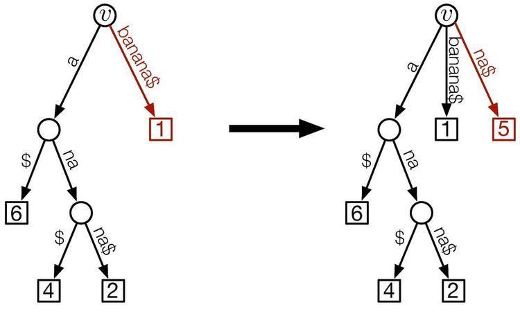
Suffix tree construction

Given the suffix array A and the LCP array H of a string S = s 1 , s 2 , . . . s n $ of length n + 1 , its suffix tree S T can be constructed in O ( n ) time based on the following idea: Start with the partial suffix tree for the lexicographically smallest suffix and repeatedly insert the other suffixes in the order given by the suffix array.

Let S T i be the partial suffix tree for 0 ≤ i ≤ n . Further let d ( v ) be the length of the concatenation of all path labels from the root of S T i to node v .

Start with S T 0 , the tree consisting only of the root. To insert A [ i + 1 ] into S T i , walk up the rightmost path beginning at the recently inserted leaf A [ i ] to the root, until the deepest node v with d ( v ) ≤ H [ i + 1 ] is reached.

We need to distinguish two cases:

1. Delete the edge ( v , w ) .
2. Add a new internal node y and a new edge ( v , y ) with label S [ A [ i ] + d ( v ) , A [ i ] + H [ i + 1 ] − 1 ] . The new label consists of the missing characters of the longest common prefix of A [ i ] and A [ i + 1 ] . Thus, the concatenation of the labels of the root-to- y path now displays the longest common prefix of A [ i ] and A [ i + 1 ] .
3. Connect w to the newly created internal node y by an edge ( y , w ) that is labeled S [ A [ i ] + H [ i + 1 ] , A [ i ] + d ( w ) − 1 ] . The new label consists of the remaining characters of the deleted edge ( v , w ) that were not used as the label of edge ( v , y ) .
4. Add A [ i + 1 ] as a new leaf x and connect it to the new internal node y by an edge ( y , x ) that is labeled S [ A [ i + 1 ] + H [ i + 1 ] , n ] . Thus the edge label consists of the remaining characters of suffix A [ i + 1 ] that are not already represented by the concatenation of the labels of the root-to- v path.
5. This creates the partial suffix tree S T i + 1 .

A simple amortization argument shows that the running time of this algorithm is bounded by O ( n ) :

The nodes that are traversed in step i by walking up the rightmost path of S T i (apart from the last node v ) are removed from the rightmost path, when A [ i + 1 ] is added to the tree as a new leaf. These nodes will never be traversed again for all subsequent steps j > i . Therefore, at most 2 n nodes will be traversed in total.

LCP queries for arbitrary suffixes

The LCP array H only contains the length of the longest common prefix of every pair of consecutive suffixes in the suffix array A . However, with the help of the inverse suffix array A − 1 ( A [ i ] = j ⇔ A − 1 [ j ] = i , i.e. the suffix S [ j , n ] that starts at position j in S is stored in position A − 1 [ j ] in A ) and constant-time range minimum queries on H , it is possible to determine the length of the longest common prefix of arbitrary suffixes in O ( 1 ) time.

Because of the lexicographic order of the suffix array, every common prefix of the suffixes S [ i , n ] and S [ j , n ] has to be a common prefix of all suffixes between i 's position in the suffix array A − 1 [ i ] and j 's position in the suffix array A − 1 [ j ] . Therefore, the length of the longest prefix that is shared by all of these suffixes is the minimum value in the interval H [ A − 1 [ i ] + 1 , A − 1 [ j ] ] . This value can be found in constant time if H is preprocessed for range minimum queries.

Thus given a string S of length n and two arbitrary positions i , j in the string S with A − 1 [ i ] < A − 1 [ j ] , the length of the longest common prefix of the suffixes S [ i , n ] and S [ j , n ] can be computed as follows: LCP ⁡ ( i , j ) = H [ RMQ H ⁡ ( A − 1 [ i ] + 1 , A − 1 [ j ] ) ] .