Jacobi elliptic functions - Alchetron, the free social encyclopedia

In mathematics, the Jacobi elliptic functions are a set of basic elliptic functions, and auxiliary theta functions, that are of historical importance. Many of their features show up in important structures and have direct relevance to some applications (e.g. the equation of a pendulum—also see pendulum (mathematics)). They also have useful analogies to the functions of trigonometry, as indicated by the matching notation sn for sin. The Jacobi elliptic functions are used more often in practical problems than the Weierstrass elliptic functions as they do not require notions of complex analysis to be defined and/or understood. They were introduced by Carl Gustav Jakob Jacobi (1829).

Introduction

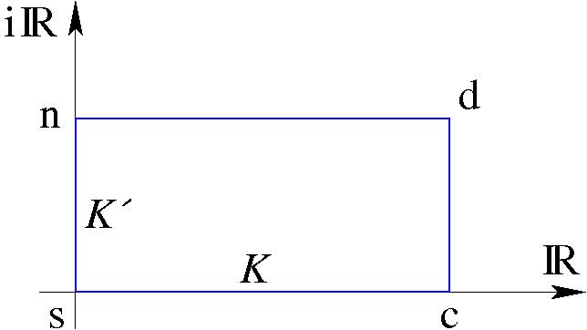
Jacobian elliptic functions are doubly periodic meromorphic functions on the complex plane. Since they are doubly periodic, they factor through a torus – in effect, their domain can be taken to be a torus, just as cosine and sine are in effect defined on a circle. Instead of having only one circle, we now have the product of two circles, one real and the other imaginary. The complex plane can be replaced by a complex torus. The circumference of the first circle is 4K and the second 4K′, where K and K′ are the quarter periods. Each function has two zeroes and two poles at opposite positions on the torus. Among the points 0, K, K + iK′, iK′ there is one zero and one pole. So an arrow can be drawn from a zero to a pole.

So there are twelve Jacobian elliptic functions. Each of the twelve corresponds to an arrow drawn from one corner of a rectangle to another. The corners of the rectangle are labeled, by convention, s, c, d and n. s is at the origin, c is at the point K on the real axis/loop, d is at the point K + iK′ and n is at point iK′ on the imaginary axis/loop. The twelve Jacobian elliptic functions are then pq, where each of p and q is a different one of the letters s, c, d, n.

The Jacobian elliptic functions are then the unique doubly periodic, meromorphic functions satisfying the following three properties:

There is a simple zero at the corner p, and a simple pole at the corner q.

The step from p to q is equal to half the period of the function pq u; that is, the function pq u is periodic in the direction pq, with the period being twice the distance from p to q. The function pq u is also periodic in the other two directions, with a period such that the distance from p to one of the other corners is a quarter period.

If the function pq u is expanded in terms of u at one of the corners, the leading term in the expansion has a coefficient of 1. In other words, the leading term of the expansion of pq u at the corner p is u; the leading term of the expansion at the corner q is 1/u, and the leading term of an expansion at the other two corners is 1.

More generally, there is no need to impose a rectangle; a parallelogram will do. However, if K and iK' are kept on the real and imaginary axis respectively, then the Jacobi elliptic functions pq u will be real functions when u is real.

Notation

The elliptic functions can be given in a variety of notations, which can make the subject unnecessarily confusing. Elliptic functions are functions of two variables. The first variable might be given in terms of the amplitude φ, or more commonly, in terms of u given below. The second variable might be given in terms of the parameter m, or as the elliptic modulus k, where k² = m, or in terms of the modular angle α, where m = sin² α. A more extensive review and definition of these alternatives, their complements, and the associated notation schemes are given in the articles on elliptic integrals and quarter period.

Definition as inverses of elliptic integrals

The above definition, in terms of the unique meromorphic functions satisfying certain properties, is quite abstract. There is a simpler, but completely equivalent definition, giving the elliptic functions as inverses of the incomplete elliptic integral of the first kind. Let

u = ∫ 0 φ d θ 1 − m sin 2 ⁡ θ .

Then the elliptic function sn u is given by

sn ⁡ u = sin ⁡ φ

and cn u is given by

cn ⁡ u = cos ⁡ φ

and

dn ⁡ u = 1 − m sin 2 ⁡ φ .

Here, the angle φ is called the amplitude. On occasion, dn u = Δ(u) is called the delta amplitude. In the above, the value m is a free parameter, usually taken to be real, 0 ≤ m ≤ 1, and so the elliptic functions can be thought of as being given by two variables, the amplitude φ and the parameter m.

The remaining nine elliptic functions are easily built from the above three, and are given in a section below.

Note that when φ = π / 2 , that u then equals the quarter period K.

Definition as trigonometry

cos ⁡ φ , sin ⁡ φ are defined on the unit circle, with radius r = 1 and angle φ = arc length of the unit circle measured from the positive x-axis. Similarly, Jacobi elliptic functions are defined on the unit ellipse, with a = 1. Let

x 2 + y 2 b 2 = 1 , b > 1 , m = 1 − 1 b 2 , 0 < m < 1 , x = r cos ⁡ φ , y = r sin ⁡ φ

then:

r ( φ , m ) = 1 1 − m 2 sin 2 ⁡ φ .

For each angle φ the angular component of the arc length, the 'angular arc length' is computed. An advantage of angular arc length is that we can calculate a total arc length for hyperbolas. For the ellipse the angular arc length is:

u = u ( φ , m ) = ∫ 0 φ r ( θ , m ) d θ .

Let P = ( x , y ) be the point on the ellipse with angular arc length u ( φ , m ) and let P ′ = ( x ′ , y ′ ) be the point on the unit circle with the angular arc length φ , (note that origin O , P ′ and P are on the same straight line). The familiar relations from the unit circle ( O P ′ = 1 ):

x ′ = cos ⁡ φ , y ′ = sin ⁡ φ

imply for the ellipse:

x ′ = cn ⁡ ( u , m ) , y ′ = sn ⁡ ( u , m ) .

So the projections of the intersection point P ′ of the line O P with the unit circle on the x- and y-axes are simply cn ⁡ ( u , m ) and sn ⁡ ( u , m ) . These projections may be interpreted as 'definition as trigonometry'. In short:

cn ⁡ ( u , m ) = x ( u , m ) r ( u , m ) , sn ⁡ ( u , m ) = y ( u , m ) r ( u , m ) , dn ⁡ ( u , m ) = 1 r ( u , m ) .

For the x and y value of the point P with u and parameter m we get, after inserting the relation:

r ( φ , m ) = 1 dn ⁡ ( u , m )

into: x = r ( φ , m ) cos ⁡ ( φ ) , y = r ( φ , m ) sin ⁡ ( φ ) that:

x = cn ⁡ ( u , m ) dn ⁡ ( u , m ) , y = sn ⁡ ( u , m ) dn ⁡ ( u , m ) .

The latter relations for the x- and y-coordinates of points on the unit ellipse may be considered as generalization of the relations x = cos ⁡ φ , y = sin ⁡ φ for the coordinates of points on the unit circle.

Introducing complex numbers, our ellipse has a dual:

x x 2 − y y 2 b 2 = 1

from applying Jacobi's imaginary transformation to the elliptic functions in the above equation for x and y.

x x = 1 dn ⁡ ( u , 1 − m ) , y y = sn ⁡ ( u , 1 − m ) dn ⁡ ( u , 1 − m )

It follows that we can put x = dn ⁡ ( u , 1 − m ) , y = sn ⁡ ( u , 1 − m ) .

Definition in terms of theta functions

Equivalently, Jacobi's elliptic functions can be defined in terms of his theta functions. If we abbreviate ϑ ( 0 ; τ ) as ϑ , and ϑ 01 ( 0 ; τ ) , ϑ 10 ( 0 ; τ ) , ϑ 11 ( 0 ; τ ) respectively as ϑ 01 , ϑ 10 , ϑ 11 (the theta constants) then the elliptic modulus k is k = ( ϑ 10 ϑ ) 2 . If we set u = π ϑ 2 z , we have

sn ⁡ ( u ; k ) = − ϑ ϑ 11 ( z ; τ ) ϑ 10 ϑ 01 ( z ; τ ) cn ⁡ ( u ; k ) = ϑ 01 ϑ 10 ( z ; τ ) ϑ 10 ϑ 01 ( z ; τ ) dn ⁡ ( u ; k ) = ϑ 01 ϑ ( z ; τ ) ϑ ϑ 01 ( z ; τ )

Since the Jacobi functions are defined in terms of the elliptic modulus k(τ), we need to invert this and find τ in terms of k. We start from k ′ = 1 − k 2 , the complementary modulus. As a function of τ it is

k ′ ( τ ) = ( ϑ 01 ϑ ) 2 .

Let us first define

ℓ = 1 2 1 − k ′ 1 + k ′ = 1 2 ϑ − ϑ 01 ϑ + ϑ 01 .

Then define the nome q as q = exp ⁡ ( π i τ ) and expand ℓ as a power series in the nome q, we obtain

ℓ = q + q 9 + q 25 + ⋯ 1 + 2 q 4 + 2 q 16 + ⋯ .

Reversion of series now gives

q = ℓ + 2 ℓ 5 + 15 ℓ 9 + 150 ℓ 13 + 1707 ℓ 17 + 20910 ℓ 21 + 268616 ℓ 25 + ⋯ .

Since we may reduce to the case where the imaginary part of τ is greater than or equal to 1/2 sqrt(3), we can assume the absolute value of q is less than or equal to exp(-1/2 sqrt(3) π) ~ 0.0658; for values this small the above series converges very rapidly and easily allows us to find the appropriate value for q.

Minor functions

Reversing the order of the two letters of the function name results in the reciprocals of the three functions above:

ns ⁡ ( u ) = 1 sn ⁡ ( u ) nc ⁡ ( u ) = 1 cn ⁡ ( u ) nd ⁡ ( u ) = 1 dn ⁡ ( u )

Similarly, the ratios of the three primary functions correspond to the first letter of the numerator followed by the first letter of the denominator:

sc ⁡ ( u ) = sn ⁡ ( u ) cn ⁡ ( u ) sd ⁡ ( u ) = sn ⁡ ( u ) dn ⁡ ( u ) dc ⁡ ( u ) = dn ⁡ ( u ) cn ⁡ ( u ) ds ⁡ ( u ) = dn ⁡ ( u ) sn ⁡ ( u ) cs ⁡ ( u ) = cn ⁡ ( u ) sn ⁡ ( u ) cd ⁡ ( u ) = cn ⁡ ( u ) dn ⁡ ( u )

More compactly, we have

pq ⁡ ( u ) = pn ⁡ ( u ) qn ⁡ ( u )

where p and q are any of the letters s, c, d.

(This notation is due to Gudermann and Glaisher and is not Jacobi's original notation

Addition theorems

The functions satisfy the two algebraic relations

cn 2 ⁡ ( u , k ) + sn 2 ⁡ ( u , k ) = 1 , dn 2 ⁡ ( u , k ) + k 2 sn 2 ⁡ ( u , k ) = 1.

From this we see that (cn, sn, dn) parametrizes an elliptic curve which is the intersection of the two quadrics defined by the above two equations. We now may define a group law for points on this curve by the addition formulas for the Jacobi functions

cn ⁡ ( x + y ) = cn ⁡ ( x ) cn ⁡ ( y ) − sn ⁡ ( x ) sn ⁡ ( y ) dn ⁡ ( x ) dn ⁡ ( y ) 1 − k 2 sn 2 ⁡ ( x ) sn 2 ⁡ ( y ) , sn ⁡ ( x + y ) = sn ⁡ ( x ) cn ⁡ ( y ) dn ⁡ ( y ) + sn ⁡ ( y ) cn ⁡ ( x ) dn ⁡ ( x ) 1 − k 2 sn 2 ⁡ ( x ) sn 2 ⁡ ( y ) , dn ⁡ ( x + y ) = dn ⁡ ( x ) dn ⁡ ( y ) − k 2 sn ⁡ ( x ) sn ⁡ ( y ) cn ⁡ ( x ) cn ⁡ ( y ) 1 − k 2 sn 2 ⁡ ( x ) sn 2 ⁡ ( y ) .

Relations between squares of the functions

− dn 2 ⁡ ( u ) + m 1 = − m cn 2 ⁡ ( u ) = m sn 2 ⁡ ( u ) − m − m 1 nd 2 ⁡ ( u ) + m 1 = − m m 1 sd 2 ⁡ ( u ) = m cd 2 ⁡ ( u ) − m m 1 sc 2 ⁡ ( u ) + m 1 = m 1 nc 2 ⁡ ( u ) = dc 2 ⁡ ( u ) − m cs 2 ⁡ ( u ) + m 1 = ds 2 ⁡ ( u ) = ns 2 ⁡ ( u ) − m

where m + m₁ = 1 and m = k².

Additional relations between squares can be obtained by noting that pq² · qp² = 1 and that pq = pr / qr where p, q, r are any of the letters s, c, d, n and ss = cc = dd = nn = 1.

Expansion in terms of the nome

Let the nome be q = exp ⁡ ( − π K ′ / K ) and let the argument be v = π u / ( 2 K ) . Then the functions have expansions as Lambert series

sn ⁡ ( u ) = 2 π K m ∑ n = 0 ∞ q n + 1 / 2 1 − q 2 n + 1 sin ⁡ ( ( 2 n + 1 ) v ) , cn ⁡ ( u ) = 2 π K m ∑ n = 0 ∞ q n + 1 / 2 1 + q 2 n + 1 cos ⁡ ( ( 2 n + 1 ) v ) , dn ⁡ ( u ) = π 2 K + 2 π K ∑ n = 1 ∞ q n 1 + q 2 n cos ⁡ ( 2 n v ) .

Jacobi elliptic functions as solutions of nonlinear ordinary differential equations

The derivatives of the three basic Jacobi elliptic functions are:

d d z sn ⁡ ( z ) = cn ⁡ ( z ) dn ⁡ ( z ) , d d z cn ⁡ ( z ) = − sn ⁡ ( z ) dn ⁡ ( z ) , d d z dn ⁡ ( z ) = − k 2 sn ⁡ ( z ) cn ⁡ ( z ) .

With the addition theorems above and for a given k with 0 < k < 1 they therefore are solutions to the following nonlinear ordinary differential equations:

sn ⁡ ( x ) solves the differential equations

and

cn ⁡ ( x ) solves the differential equations

and

dn ⁡ ( x ) solves the differential equations

and

Approximation in terms of hyperbolic functions

The Jacobi elliptic functions can be expanded in terms of the hyperbolic functions. When m is close to unit such that m 1 2 and higher power of m 1 can be neglected we have

sn(u):

cn(u):

dn(u):

am(u):

Inverse functions

The inverses of the Jacobi elliptic functions can be defined similarly to the inverse trigonometric functions; if x = sn ⁡ ( ξ , k ) , ξ = a r c s n ( x , k ) . They can be represented as elliptic integrals, and power series representations have been found.