Theta function - Alchetron, The Free Social Encyclopedia

In mathematics, theta functions are special functions of several complex variables. They are important in many areas, including the theories of Abelian varieties and moduli spaces, and of quadratic forms. They have also been applied to soliton theory. When generalized to a Grassmann algebra, they also appear in quantum field theory.

The most common form of theta function is that occurring in the theory of elliptic functions. With respect to one of the complex variables (conventionally called z), a theta function has a property expressing its behavior with respect to the addition of a period of the associated elliptic functions, making it a quasiperiodic function. In the abstract theory this comes from a line bundle condition of descent.

Jacobi theta function

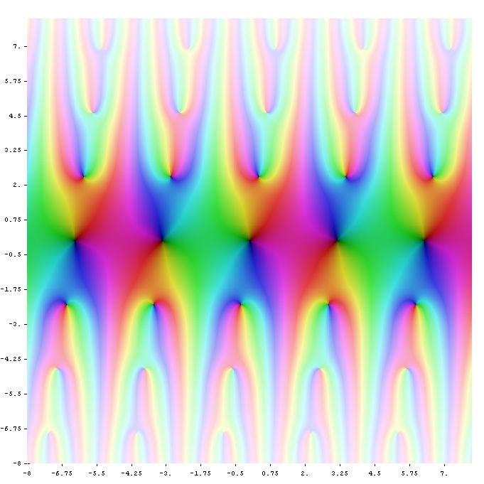
There are several closely related functions called Jacobi theta functions, and many different and incompatible systems of notation for them. One Jacobi theta function (named after Carl Gustav Jacob Jacobi) is a function defined for two complex variables z and τ, where z can be any complex number and τ is confined to the upper half-plane, which means it has positive imaginary part. It is given by the formula

ϑ ( z ; τ ) = ∑ n = − ∞ ∞ exp ⁡ ( π i n 2 τ + 2 π i n z ) = 1 + 2 ∑ n = 1 ∞ ( e π i τ ) n 2 cos ⁡ ( 2 π n z ) = ∑ n = − ∞ ∞ q n 2 η n

where q = exp(πiτ) and η = exp(2πiz). It is a Jacobi form. If τ is fixed, this becomes a Fourier series for a periodic entire function of z with period 1; in this case, the theta function satisfies the identity

ϑ ( z + 1 ; τ ) = ϑ ( z ; τ ) .

The function also behaves very regularly with respect to its quasi-period τ and satisfies the functional equation

ϑ ( z + a + b τ ; τ ) = exp ⁡ ( − π i b 2 τ − 2 π i b z ) ϑ ( z ; τ )

where a and b are integers.

Auxiliary functions

The Jacobi theta function defined above is sometimes considered along with three auxiliary theta functions, in which case it is written with a double 0 subscript:

ϑ 00 ( z ; τ ) = ϑ ( z ; τ )

The auxiliary (or half-period) functions are defined by

ϑ 01 ( z ; τ ) = ϑ ( z + 1 2 ; τ ) ϑ 10 ( z ; τ ) = exp ⁡ ( 1 4 π i τ + π i z ) ϑ ( z + 1 2 τ ; τ ) ϑ 11 ( z ; τ ) = exp ⁡ ( 1 4 π i τ + π i ( z + 1 2 ) ) ϑ ( z + 1 2 τ + 1 2 ; τ ) .

This notation follows Riemann and Mumford; Jacobi's original formulation was in terms of the nome q = e^iπτ rather than τ. In Jacobi's notation the θ-functions are written:

θ 1 ( z ; q ) = − ϑ 11 ( z ; τ ) θ 2 ( z ; q ) = ϑ 10 ( z ; τ ) θ 3 ( z ; q ) = ϑ 00 ( z ; τ ) θ 4 ( z ; q ) = ϑ 01 ( z ; τ )

The above definitions of the Jacobi theta functions are by no means unique. See Jacobi theta functions (notational variations) for further discussion.

If we set z = 0 in the above theta functions, we obtain four functions of τ only, defined on the upper half-plane (sometimes called theta constants.) These can be used to define a variety of modular forms, and to parametrize certain curves; in particular, the Jacobi identity is

ϑ 00 ( 0 ; τ ) 4 = ϑ 01 ( 0 ; τ ) 4 + ϑ 10 ( 0 ; τ ) 4

which is the Fermat curve of degree four.

Jacobi identities

Jacobi's identities describe how theta functions transform under the modular group, which is generated by τ ↦ τ + 1 and τ ↦ −1/τ. Equations for the first transform are easily found since adding one to τ in the exponent has the same effect as adding 1/2 to z (n ≡ n² mod 2). For the second, let

α = ( − i τ ) 1 2 exp ⁡ ( π τ i z 2 ) .

Then

ϑ 00 ( z τ ; − 1 τ ) = α ϑ 00 ( z ; τ ) ϑ 01 ( z τ ; − 1 τ ) = α ϑ 10 ( z ; τ ) ϑ 10 ( z τ ; − 1 τ ) = α ϑ 01 ( z ; τ ) ϑ 11 ( z τ ; − 1 τ ) = − i α ϑ 11 ( z ; τ ) .

Theta functions in terms of the nome

Instead of expressing the Theta functions in terms of z and τ, we may express them in terms of arguments w and the nome q, where w = e^πiz and q = e^πiτ. In this form, the functions become

ϑ 00 ( w , q ) = ∑ n = − ∞ ∞ ( w 2 ) n q n 2 ϑ 01 ( w , q ) = ∑ n = − ∞ ∞ ( − 1 ) n ( w 2 ) n q n 2 ϑ 10 ( w , q ) = ∑ n = − ∞ ∞ ( w 2 ) n + 1 2 q ( n + 1 2 ) 2 ϑ 11 ( w , q ) = i ∑ n = − ∞ ∞ ( − 1 ) n ( w 2 ) n + 1 2 q ( n + 1 2 ) 2 .

We see that the theta functions can also be defined in terms of w and q, without a direct reference to the exponential function. These formulas can, therefore, be used to define the Theta functions over other fields where the exponential function might not be everywhere defined, such as fields of p-adic numbers.

Product representations

The Jacobi triple product tells us that for complex numbers w and q with | q | < 1 and w ≠ 0 we have

∏ m = 1 ∞ ( 1 − q 2 m ) ( 1 + w 2 q 2 m − 1 ) ( 1 + w − 2 q 2 m − 1 ) = ∑ n = − ∞ ∞ w 2 n q n 2 .

It can be proven by elementary means, as for instance in Hardy and Wright's An Introduction to the Theory of Numbers.

If we express the theta function in terms of the nome q = e^πiτ and w = e^πiz then

ϑ ( z ; τ ) = ∑ n = − ∞ ∞ exp ⁡ ( π i τ n 2 ) exp ⁡ ( 2 π i z n ) = ∑ n = − ∞ ∞ w 2 n q n 2 .

We therefore obtain a product formula for the theta function in the form

ϑ ( z ; τ ) = ∏ m = 1 ∞ ( 1 − exp ⁡ ( 2 m π i τ ) ) ( 1 + exp ⁡ ( ( 2 m − 1 ) π i τ + 2 π i z ) ) ( 1 + exp ⁡ ( ( 2 m − 1 ) π i τ − 2 π i z ) ) .

In terms of w and q:

ϑ ( z ; τ ) = ∏ m = 1 ∞ ( 1 − q 2 m ) ( 1 + q 2 m − 1 w 2 ) ( 1 + q 2 m − 1 w 2 ) = ( q 2 ; q 2 ) ∞ ( − w 2 q ; q 2 ) ∞ ( − q w 2 ; q 2 ) ∞ = ( q 2 ; q 2 ) ∞ θ ( − w 2 q ; q 2 )

where ( ; )_∞ is the q-Pochhammer symbol and θ( ; ) is the q-theta function. Expanding terms out, the Jacobi triple product can also be written

∏ m = 1 ∞ ( 1 − q 2 m ) ( 1 + ( w 2 + w − 2 ) q 2 m − 1 + q 4 m − 2 ) ,

which we may also write as

ϑ ( z ∣ q ) = ∏ m = 1 ∞ ( 1 − q 2 m ) ( 1 + 2 cos ⁡ ( 2 π z ) q 2 m − 1 + q 4 m − 2 ) .

This form is valid in general but clearly is of particular interest when z is real. Similar product formulas for the auxiliary theta functions are

ϑ 01 ( z ∣ q ) = ∏ m = 1 ∞ ( 1 − q 2 m ) ( 1 − 2 cos ⁡ ( 2 π z ) q 2 m − 1 + q 4 m − 2 ) , ϑ 10 ( z ∣ q ) = 2 q 1 4 cos ⁡ ( π z ) ∏ m = 1 ∞ ( 1 − q 2 m ) ( 1 + 2 cos ⁡ ( 2 π z ) q 2 m + q 4 m ) , ϑ 11 ( z ∣ q ) = − 2 q 1 4 sin ⁡ ( π z ) ∏ m = 1 ∞ ( 1 − q 2 m ) ( 1 − 2 cos ⁡ ( 2 π z ) q 2 m + q 4 m ) .

Integral representations

The Jacobi theta functions have the following integral representations:

ϑ 00 ( z ; τ ) = − i ∫ i − ∞ i + ∞ e i π τ u 2 cos ⁡ ( 2 u z + π u ) sin ⁡ ( π u ) d u ; ϑ 01 ( z ; τ ) = − i ∫ i − ∞ i + ∞ e i π τ u 2 cos ⁡ ( 2 u z ) sin ⁡ ( π u ) d u ; ϑ 10 ( z ; τ ) = − i e i z + 1 4 i π τ ∫ i − ∞ i + ∞ e i π τ u 2 cos ⁡ ( 2 u z + π u + π τ u ) sin ⁡ ( π u ) d u ; ϑ 11 ( z ; τ ) = e i z + 1 4 i π τ ∫ i − ∞ i + ∞ e i π τ u 2 cos ⁡ ( 2 u z + π τ u ) sin ⁡ ( π u ) d u .

Explicit values

See Yi (2004).

φ ( e − π x ) = ϑ ( 0 ; i x ) = θ 3 ( 0 ; e − π x ) = ∑ n = − ∞ ∞ e − x π n 2 φ ( e − π ) = π 4 Γ ( 3 4 ) φ ( e − 2 π ) = 6 π + 4 2 π 4 2 Γ ( 3 4 ) φ ( e − 3 π ) = 27 π + 18 3 π 4 3 Γ ( 3 4 ) φ ( e − 4 π ) = 8 π 4 + 2 π 4 4 Γ ( 3 4 ) φ ( e − 5 π ) = 225 π + 100 5 π 4 5 Γ ( 3 4 ) φ ( e − 6 π ) = 3 2 + 3 3 4 + 2 3 − 27 4 + 1728 4 − 4 3 ⋅ 243 π 2 8 6 1 + 6 − 2 − 3 6 Γ ( 3 4 )

Some series identities

The next two series identities were proved by István Mező:

ϑ 4 2 ( q ) = i q 1 4 ∑ k = − ∞ ∞ q 2 k 2 − k ϑ 1 ( 2 k − 1 2 i ln ⁡ q , q ) , ϑ 4 2 ( q ) = ∑ k = − ∞ ∞ q 2 k 2 ϑ 4 ( k ln ⁡ q i , q ) .

These relations hold for all 0 < q < 1. Specializing the values of q, we have the next parameter free sums

π e π 2 ⋅ 1 Γ 2 ( 3 4 ) = i ∑ k = − ∞ ∞ e π ( k − 2 k 2 ) ϑ 1 ( i π 2 ( 2 k − 1 ) , e − π ) , π 2 ⋅ 1 Γ 2 ( 3 4 ) = ∑ k = − ∞ ∞ ϑ 4 ( i k π , e − π ) e 2 π k 2

Zeros of the Jacobi theta functions

All zeros of the Jacobi theta functions are simple zeros and are given by the following:

ϑ ( z , τ ) = ϑ 3 ( z , τ ) = 0 ⟺ z = m + n τ + 1 2 + τ 2 ϑ 1 ( z , τ ) = 0 ⟺ z = m + n τ ϑ 2 ( z , τ ) = 0 ⟺ z = m + n τ + 1 2 ϑ 4 ( z , τ ) = 0 ⟺ z = m + n τ + τ 2

where m, n are arbitrary integers.

Relation to the Riemann zeta function

The relation

ϑ ( 0 ; − 1 τ ) = ( − i τ ) 1 2 ϑ ( 0 ; τ )

was used by Riemann to prove the functional equation for the Riemann zeta function, by means of the integral

Γ ( s 2 ) π − s 2 ζ ( s ) = 1 2 ∫ 0 ∞ ( ϑ ( 0 ; i t ) − 1 ) t s 2 d t t

which can be shown to be invariant under substitution of s by 1 − s. The corresponding integral for z ≠ 0 is given in the article on the Hurwitz zeta function.

Relation to the Weierstrass elliptic function

The theta function was used by Jacobi to construct (in a form adapted to easy calculation) his elliptic functions as the quotients of the above four theta functions, and could have been used by him to construct Weierstrass's elliptic functions also, since

℘ ( z ; τ ) = − ( log ⁡ ϑ 11 ( z ; τ ) ) ″ + c

where the second derivative is with respect to z and the constant c is defined so that the Laurent expansion of ℘(z) at z = 0 has zero constant term.

Relation to the q-gamma function

The fourth theta function – and thus the others too – is intimately connected to the Jackson q-gamma function via the relation

( Γ q 2 ( x ) Γ q 2 ( 1 − x ) ) − 1 = q 2 x ( 1 − x ) ( q − 2 ; q − 2 ) ∞ 3 ( q 2 − 1 ) ϑ 4 ( 1 2 i ( 1 − 2 x ) log ⁡ q , 1 q ) .

Relations to Dedekind eta function

Let η(τ) be the Dedekind eta function, and the argument of the theta function as the nome q = e^πiτ. Then,

θ 2 ( 0 , q ) = ϑ 10 ( 0 ; τ ) = 2 η 2 ( 2 τ ) η ( τ ) , θ 3 ( 0 , q ) = ϑ 00 ( 0 ; τ ) = η 5 ( τ ) η 2 ( 1 2 τ ) η 2 ( 2 τ ) = η 2 ( 1 2 ( τ + 1 ) ) η ( τ + 1 ) , θ 4 ( 0 , q ) = ϑ 01 ( 0 ; τ ) = η 2 ( 1 2 τ ) η ( τ ) ,

and,

θ 2 ( 0 , q ) θ 3 ( 0 , q ) θ 4 ( 0 , q ) = 2 η 3 ( τ ) .

Elliptic modulus

The elliptic modulus is

k ( τ ) = ϑ 10 ( 0 , τ ) 2 ϑ 00 ( 0 , τ ) 2

and the complementary elliptic modulus is

k ′ ( τ ) = ϑ 01 ( 0 , τ ) 2 ϑ 00 ( 0 , τ ) 2

A solution to the heat equation

The Jacobi theta function is the fundamental solution of the one-dimensional heat equation with spatially periodic boundary conditions. Taking z = x to be real and τ = it with t real and positive, we can write

ϑ ( x , i t ) = 1 + 2 ∑ n = 1 ∞ exp ⁡ ( − π n 2 t ) cos ⁡ ( 2 π n x )

which solves the heat equation

∂ ∂ t ϑ ( x , i t ) = 1 4 π ∂ 2 ∂ x 2 ϑ ( x , i t ) .

This theta-function solution is 1-periodic in x, and as t → 0 it approaches the periodic delta function, or Dirac comb, in the sense of distributions

lim t → 0 ϑ ( x , i t ) = ∑ n = − ∞ ∞ δ ( x − n ) .

General solutions of the spatially periodic initial value problem for the heat equation may be obtained by convolving the initial data at t = 0 with the theta function.

Relation to the Heisenberg group

The Jacobi theta function is invariant under the action of a discrete subgroup of the Heisenberg group. This invariance is presented in the article on the theta representation of the Heisenberg group.

Generalizations

If F is a quadratic form in n variables, then the theta function associated with F is

θ F ( z ) = ∑ m ∈ Z n e 2 π i z F ( m )

with the sum extending over the lattice of integers ℤⁿ. This theta function is a modular form of weight n/2 (on an appropriately defined subgroup) of the modular group. In the Fourier expansion,

θ ^ F ( z ) = ∑ k = 0 ∞ R F ( k ) e 2 π i k z ,

the numbers R_F(k) are called the representation numbers of the form.

Riemann theta function

Let

H n = { F ∈ M ( n , C ) | F = F T , Im ⁡ F > 0 }

the set of symmetric square matrices whose imaginary part is positive definite. ℍ_n is called the Siegel upper half-space and is the multi-dimensional analog of the upper half-plane. The n-dimensional analogue of the modular group is the symplectic group Sp(2n,ℤ); for n = 1, Sp(2,ℤ) = SL(2,ℤ). The n-dimensional analogue of the congruence subgroups is played by

ker ⁡ { Sp ⁡ ( 2 n , Z ) → Sp ⁡ ( 2 n , Z / k Z ) } .

Then, given τ ∈ ℍ_n, the Riemann theta function is defined as

θ ( z , τ ) = ∑ m ∈ Z n exp ⁡ ( 2 π i ( 1 2 m T τ m + m T z ) ) .

Here, z ∈ ℂⁿ is an n-dimensional complex vector, and the superscript T denotes the transpose. The Jacobi theta function is then a special case, with n = 1 and τ ∈ ℍ where ℍ is the upper half-plane.

The Riemann theta converges absolutely and uniformly on compact subsets of ℂⁿ × ℍ_n.

The functional equation is

θ ( z + a + τ b , τ ) = exp ⁡ 2 π i ( − b T z − 1 2 b T τ b ) θ ( z , τ )

which holds for all vectors a, b ∈ ℤⁿ, and for all z ∈ ℂⁿ and τ ∈ ℍ_n.

Poincaré series

The Poincaré series generalizes the theta series to automorphic forms with respect to arbitrary Fuchsian groups.

References

Theta function Wikipedia

(Text) CC BY-SA

Contents