Iterative deepening depth first search

Algorithm

The following pseudocode shows IDDFS implemented in terms of a recursive depth-limited DFS (called DLS).

function IDDFS(root) for depth from 0 to ∞ found ← DLS(root, depth) if found ≠ null return found function DLS(node, depth) if depth = 0 and node is a goal return node if depth > 0 foreach child of node found ← DLS(child, depth−1) if found ≠ null return found return null

Properties

IDDFS combines depth-first search's space-efficiency and breadth-first search's completeness (when the branching factor is finite). It is optimal when the path cost is a non-decreasing function of the depth of the node.

Since iterative deepening visits states multiple times, it may seem wasteful, but it turns out to be not so costly, since in a tree most of the nodes are in the bottom level, so it does not matter much if the upper levels are visited multiple times.

The main advantage of IDDFS in game tree searching is that the earlier searches tend to improve the commonly used heuristics, such as the killer heuristic and alpha-beta pruning, so that a more accurate estimate of the score of various nodes at the final depth search can occur, and the search completes more quickly since it is done in a better order. For example, alpha-beta pruning is most efficient if it searches the best moves first.

A second advantage is the responsiveness of the algorithm. Because early iterations use small values for d , they execute extremely quickly. This allows the algorithm to supply early indications of the result almost immediately, followed by refinements as d increases. When used in an interactive setting, such as in a chess-playing program, this facility allows the program to play at any time with the current best move found in the search it has completed so far. This can be phrased as each depth of the search corecursively producing a better approximation of the solution, though the work done at each step is recursive. This is not possible with a traditional depth-first search, which does not produce intermediate results.

Time complexity

The time complexity of IDDFS in a (well-balanced) tree works out to be the same as depth-first search, i.e. O ( b d ) , where b is the branching factor and d is the depth of the goal.

Proof

In an iterative deepening search, the nodes at depth d are expanded once, those at depth d − 1 are expanded twice, and so on up to the root of the search tree, which is expanded d + 1 times. So the total number of expansions in an iterative deepening search is

b d + 2 b d − 1 + 3 b d − 2 + ⋯ + ( d − 1 ) b 2 + d b + ( d + 1 ) = ∑ i = 0 d ( d + 1 − i ) b i

where b d is the number of times the nodes at depth d are visited, 2 b d − 1 is the number of times the nodes at depth d − 1 are visited, and so on. Factoring out b d gives

b d ( 1 + 2 b − 1 + 3 b − 2 + ⋯ + ( d − 1 ) b 2 − d + d b 1 − d + ( d + 1 ) b − d )

Now let x = 1 b = b − 1 . Then we have

b d ( 1 + 2 x + 3 x 2 + ⋯ + ( d − 1 ) x d − 2 + d x d − 1 + ( d + 1 ) x d )

This is less than the infinite series

b d ( 1 + 2 x + 3 x 2 + 4 x 3 + ⋯ ) = b d ( ∑ n = 1 ∞ n x n − 1 )

which converges to

b d ( 1 − x ) − 2 = b d 1 ( 1 − x ) 2 , for a b s ( x ) < 1

That is, we have

b d ( 1 + 2 x + 3 x 2 + ⋯ + ( d − 1 ) x d − 2 + d x d − 1 + ( d + 1 ) x d ) ≤ b d ( 1 − x ) − 2 , for a b s ( x ) < 1

Since ( 1 − x ) − 2 or ( 1 − 1 b ) − 2 is a constant independent of d (the depth), if b > 1 (i.e., if the branching factor is greater than 1), the running time of the depth-first iterative deepening search is O ( b d ) .

Example

For b = 10 and d = 5 the number is

∑ i = 0 5 ( 5 + 1 − i ) 10 i = 6 + 50 + 400 + 3000 + 20000 + 100000 = 123456

All together, an iterative deepening search from depth 1 all the way down to depth d expands only about 11 % more nodes than a single breadth-first or depth-limited search to depth d , when b = 10 .

The higher the branching factor, the lower the overhead of repeatedly expanded states, but even when the branching factor is 2, iterative deepening search only takes about twice as long as a complete breadth-first search. This means that the time complexity of iterative deepening is still O ( b d ) .

Space complexity

The space complexity of IDDFS is O ( d ) , where d is the depth of the goal.

Proof

Since IDDFS, at any point, is engaged in a depth-first search, it need only store a stack of nodes which represents the branch of the tree it is expanding. Since it finds a solution of optimal length, the maximum depth of this stack is d , and hence the maximum amount of space is O ( d ) .

In general, iterative deepening is the preferred search method when there is a large search space and the depth of the solution is not known.

Example

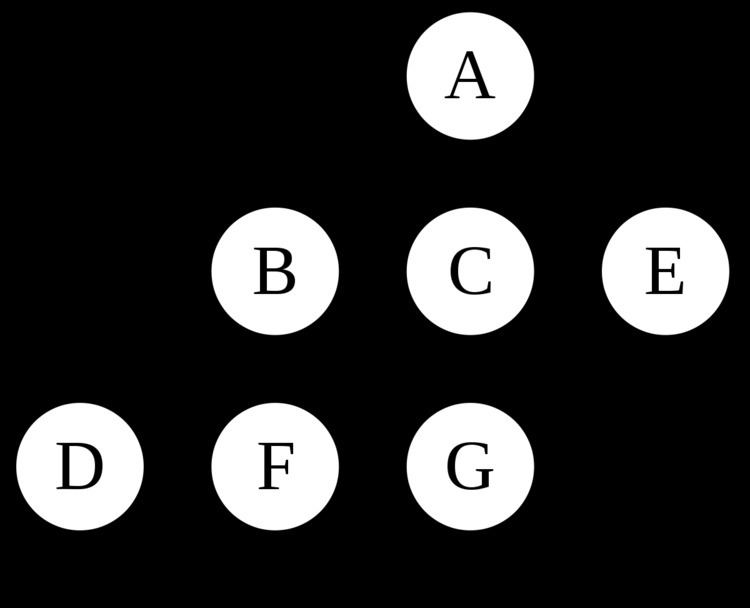
For the following graph:

a depth-first search starting at A, assuming that the left edges in the shown graph are chosen before right edges, and assuming the search remembers previously-visited nodes and will not repeat them (since this is a small graph), will visit the nodes in the following order: A, B, D, F, E, C, G. The edges traversed in this search form a Trémaux tree, a structure with important applications in graph theory.

Performing the same search without remembering previously visited nodes results in visiting nodes in the order A, B, D, F, E, A, B, D, F, E, etc. forever, caught in the A, B, D, F, E cycle and never reaching C or G.

Iterative deepening prevents this loop and will reach the following nodes on the following depths, assuming it proceeds left-to-right as above:

0: A

1: A, B, C, E

(Note that iterative deepening has now seen C, when a conventional depth-first search did not.)

2: A, B, D, F, C, G, E, F

(Note that it still sees C, but that it came later. Also note that it sees E via a different path, and loops back to F twice.)

3: A, B, D, F, E, C, G, E, F, B

For this graph, as more depth is added, the two cycles "ABFE" and "AEFB" will simply get longer before the algorithm gives up and tries another branch.

Related algorithms

Similar to iterative deepening is a search strategy called iterative lengthening search that works with increasing path-cost limits instead of depth-limits. It expands nodes in the order of increasing path cost; therefore the first goal it encounters is the one with the cheapest path cost. But iterative lengthening incurs substantial overhead that makes it less useful than iterative deepening.

Iterative deepening A* is a best-first search that performs iterative deepening based on "f"-values similar to the ones computed in the A* algorithm.