
 | ||
Worst-case performance O ( | V | + | E | ) = O ( b d ) {displaystyle O(|V|+|E|)=O(b^{d})} Worst-case space complexity O ( | V | ) = O ( b d ) {displaystyle O(|V|)=O(b^{d})} | ||
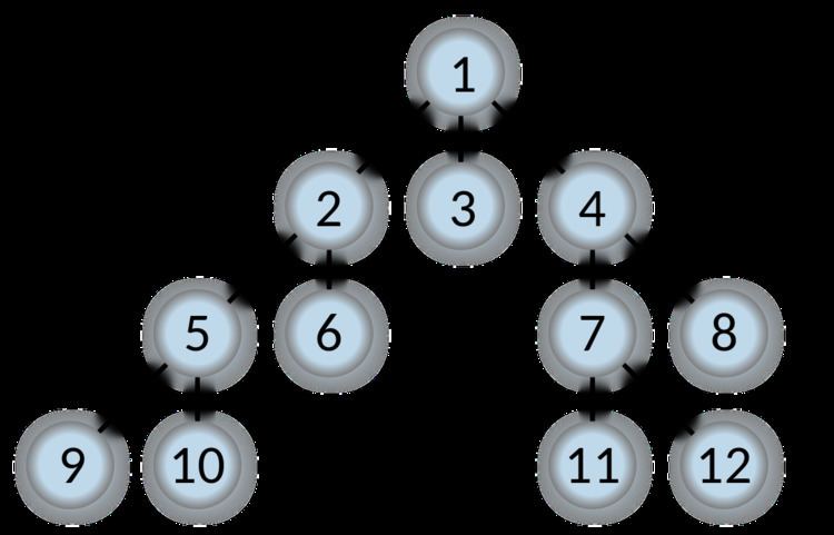
Breadth-first search (BFS) is an algorithm for traversing or searching tree or graph data structures. It starts at the tree root (or some arbitrary node of a graph, sometimes referred to as a 'search key') and explores the neighbor nodes first, before moving to the next level neighbors.
Contents
- Pseudocode
- More details
- Example
- Time and space complexity
- Completeness and optimality
- BFS ordering
- Applications
- References
BFS was invented in the late 1950s by E. F. Moore, who used it to find the shortest path out of a maze, and discovered independently by C. Y. Lee as a wire routing algorithm (published 1961).
Pseudocode
Input: A graph Graph and a starting vertex root of Graph
Output: Goal state. The parent links trace the shortest path back to root
A non-recursive implementation of breadth-first search:
More details
This non-recursive implementation is similar to the non-recursive implementation of depth-first search, but differs from it in two ways:
- it uses a queue (First In First Out) instead of a stack and
- it checks whether a vertex has been discovered before enqueueing the vertex rather than delaying this check until the vertex is dequeued from the queue.
The Q queue contains the frontier along which the algorithm is currently searching.
The S set is used to track which vertices have been visited (required for a general graph search, but not for a tree search). At the beginning of the algorithm, the set is empty. At the end of the algorithm, it contains all vertices with a distance from root less than the goal.
The parent attribute of each vertex is useful for accessing the nodes in a shortest path, for example by backtracking from the destination node up to the starting node, once the BFS has been run, and the predecessors nodes have been set.
The NIL is just a symbol that represents the absence of something, in this case it represents the absence of a parent (or predecessor) node; sometimes instead of the word NIL, words such as null, none or nothing can also be used.
Note that the word node is usually interchangeable with the word vertex.
Breadth-first search produces a so-called breadth first tree. You can see how a breadth first tree looks in the following example.
Example
The following is an example of the breadth-first tree obtained by running a BFS starting from Frankfurt:
Time and space complexity
The time complexity can be expressed as
When the number of vertices in the graph is known ahead of time, and additional data structures are used to determine which vertices have already been added to the queue, the space complexity can be expressed as
When working with graphs that are too large to store explicitly (or infinite), it is more practical to describe the complexity of breadth-first search in different terms: to find the nodes that are at distance d from the start node (measured in number of edge traversals), BFS takes O(bd + 1) time and memory, where b is the "branching factor" of the graph (the average out-degree).
Completeness and optimality
In the analysis of algorithms, the input to breadth-first search is assumed to be a finite graph, represented explicitly as an adjacency list or similar representation. However, in the application of graph traversal methods in artificial intelligence the input may be an implicit representation of an infinite graph. In this context, a search method is described as being complete if it is guaranteed to find a goal state if one exists. Breadth-first search is complete, but depth-first search is not. When applied to infinite graphs represented implicitly, breadth-first search will eventually find the goal state, but depth-first search may get lost in parts of the graph that have no goal state and never return.
BFS ordering
An enumeration of the vertices of a graph is said to be a BFS ordering if it is the possible output of the application of BFS to this graph.
Let
Let
Applications
Breadth-first search can be used to solve many problems in graph theory, for example: