
Data structure Graph | ||
 | ||
Worst-case performance O ( | V | + | E | ) {displaystyle O(|V|+|E|)} for explicit graphs traversed without repetition, O ( b d ) {displaystyle O(b^{d})} for implicit graphs with branching factor b searched to depth d Worst-case space complexity O ( | V | ) {displaystyle O(|V|)} if entire graph is traversed without repetition, O(longest path length searched) for implicit graphs without elimination of duplicate nodes | ||
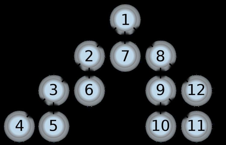
Depth-first search (DFS) is an algorithm for traversing or searching tree or graph data structures. One starts at the root (selecting some arbitrary node as the root in the case of a graph) and explores as far as possible along each branch before backtracking.
Contents
- Properties
- Example
- Output of a depth first search
- DFS ordering
- Vertex orderings
- Pseudocode
- Applications
- Complexity
- References
A version of depth-first search was investigated in the 19th century by French mathematician Charles Pierre Trémaux as a strategy for solving mazes.
Properties
The time and space analysis of DFS differs according to its application area. In theoretical computer science, DFS is typically used to traverse an entire graph, and takes time Θ(|V| + |E|), linear in the size of the graph. In these applications it also uses space O(|V|) in the worst case to store the stack of vertices on the current search path as well as the set of already-visited vertices. Thus, in this setting, the time and space bounds are the same as for breadth-first search and the choice of which of these two algorithms to use depends less on their complexity and more on the different properties of the vertex orderings the two algorithms produce.
For applications of DFS in relation to specific domains, such as searching for solutions in artificial intelligence or web-crawling, the graph to be traversed is often either too large to visit in its entirety or infinite (DFS may suffer from non-termination). In such cases, search is only performed to a limited depth; due to limited resources, such as memory or disk space, one typically does not use data structures to keep track of the set of all previously visited vertices. When search is performed to a limited depth, the time is still linear in terms of the number of expanded vertices and edges (although this number is not the same as the size of the entire graph because some vertices may be searched more than once and others not at all) but the space complexity of this variant of DFS is only proportional to the depth limit, and as a result, is much smaller than the space needed for searching to the same depth using breadth-first search. For such applications, DFS also lends itself much better to heuristic methods for choosing a likely-looking branch. When an appropriate depth limit is not known a priori, iterative deepening depth-first search applies DFS repeatedly with a sequence of increasing limits. In the artificial intelligence mode of analysis, with a branching factor greater than one, iterative deepening increases the running time by only a constant factor over the case in which the correct depth limit is known due to the geometric growth of the number of nodes per level.
DFS may also be used to collect a sample of graph nodes. However, incomplete DFS, similarly to incomplete BFS, is biased towards nodes of high degree.
Example
For the following graph:
a depth-first search starting at A, assuming that the left edges in the shown graph are chosen before right edges, and assuming the search remembers previously visited nodes and will not repeat them (since this is a small graph), will visit the nodes in the following order: A, B, D, F, E, C, G. The edges traversed in this search form a Trémaux tree, a structure with important applications in graph theory.
Performing the same search without remembering previously visited nodes results in visiting nodes in the order A, B, D, F, E, A, B, D, F, E, etc. forever, caught in the A, B, D, F, E cycle and never reaching C or G.
Iterative deepening is one technique to avoid this infinite loop and would reach all nodes.
Output of a depth-first search
A convenient description of a depth first search of a graph is in terms of a spanning tree of the vertices reached during the search. Based on this spanning tree, the edges of the original graph can be divided into three classes: forward edges, which point from a node of the tree to one of its descendants, back edges, which point from a node to one of its ancestors, and cross edges, which do neither. Sometimes tree edges, edges which belong to the spanning tree itself, are classified separately from forward edges. If the original graph is undirected then all of its edges are tree edges or back edges.
DFS ordering
An enumeration of the vertices of a graph is said to be a DFS ordering if it is the possible output of the application of DFS to this graph.
Let
Let
Vertex orderings
It is also possible to use the depth-first search to linearly order the vertices of the original graph (or tree). There are three common ways of doing this:
Pseudocode
Input: A graph G and a vertex v of G
Output: All vertices reachable from v labeled as discovered
A recursive implementation of DFS:
1 procedure DFS(G,v):2 label v as discovered3 for all edges from v to w in G.adjacentEdges(v) do4 if vertex w is not labeled as discovered then5 recursively call DFS(G,w)A non-recursive implementation of DFS:
1 procedure DFS-iterative(G,v):2 let S be a stack3 S.push(v)4 while S is not empty5 v = S.pop()6 if v is not labeled as discovered:7 label v as discovered8 for all edges from v to w in G.adjacentEdges(v) do 9 S.push(w)These two variations of DFS visit the neighbors of each vertex in the opposite order from each other: the first neighbor of v visited by the recursive variation is the first one in the list of adjacent edges, while in the iterative variation the first visited neighbor is the last one in the list of adjacent edges. The recursive implementation will visit the nodes from the example graph in the following order: A, B, D, F, E, C, G. The non-recursive implementation will visit the nodes as: A, E, F, B, D, C, G.
The non-recursive implementation is similar to breadth-first search but differs from it in two ways:
- it uses a stack instead of a queue, and
- it delays checking whether a vertex has been discovered until the vertex is popped from the stack rather than making this check before pushing the vertex.
Note that this non-recursive implementation of DFS may use O(|E|) space in the worst case, for example on a complete graph.
Applications
Algorithms that use depth-first search as a building block include:
Complexity
The computational complexity of DFS was investigated by John Reif, who showed that a decision version of it (establish whether some vertex u occurs before some vertex v in a DFS order of a rooted graph) is P-complete, meaning that it is "a nightmare for parallel processing".