Hough transform

History

It was initially invented for machine analysis of bubble chamber photographs (Hough, 1959).

The Hough transform was patented as U.S. Patent 3,069,654 in 1962 and assigned to the U.S. Atomic Energy Commission with the name "Method and Means for Recognizing Complex Patterns". This patent uses a slope-intercept parametrization for straight lines, which awkwardly leads to an unbounded transform space since the slope can go to infinity.

The rho-theta parametrization universally used today was first described in

Duda, R. O. and P. E. Hart, "Use of the Hough Transformation to Detect Lines and Curves in Pictures," Comm. ACM, Vol. 15, pp. 11–15 (January, 1972),

although it was already standard for the Radon transform since at least the 1930s.

O'Gorman and Clowes' variation is described in

O'Gorman, Frank; Clowes, MB (1976). "Finding Picture Edges Through Collinearity of Feature Points". IEEE Trans. Comput. 25 (4): 449–456. 

The story of how the modern form of the Hough transform was invented is given in

Hart, P. E., "How the Hough Transform was Invented" (PDF, 268 kB), IEEE Signal Processing Magazine, Vol 26, Issue 6, pp 18 – 22 (November, 2009).

Theory

In automated analysis of digital images, a subproblem often arises of detecting simple shapes, such as straight lines, circles or ellipses. In many cases an edge detector can be used as a pre-processing stage to obtain image points or image pixels that are on the desired curve in the image space. Due to imperfections in either the image data or the edge detector, however, there may be missing points or pixels on the desired curves as well as spatial deviations between the ideal line/circle/ellipse and the noisy edge points as they are obtained from the edge detector. For these reasons, it is often non-trivial to group the extracted edge features to an appropriate set of lines, circles or ellipses. The purpose of the Hough transform is to address this problem by making it possible to perform groupings of edge points into object candidates by performing an explicit voting procedure over a set of parameterized image objects (Shapiro and Stockman, 304).

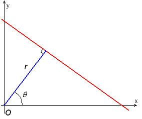
The simplest case of Hough transform is detecting straight lines. In general, the straight line y = mx + b can be represented as a point (b, m) in the parameter space. However, vertical lines pose a problem. They would give rise to unbounded values of the slope parameter m. Thus, for computational reasons, Duda and Hart proposed the use of the Hesse normal form

r = x cos ⁡ θ + y sin ⁡ θ ,

where r is the distance from the origin to the closest point on the straight line, and θ (theta) is the angle between the x axis and the line connecting the origin with that closest point.

It is therefore possible to associate with each line of the image a pair ( r , θ ) . The ( r , θ ) plane is sometimes referred to as Hough space for the set of straight lines in two dimensions. This representation makes the Hough transform conceptually very close to the two-dimensional Radon transform. (They can be seen as different ways of looking at the same transform.)

Given a single point in the plane, then the set of all straight lines going through that point corresponds to a sinusoidal curve in the (r,θ) plane, which is unique to that point. A set of two or more points that form a straight line will produce sinusoids which cross at the (r,θ) for that line. Thus, the problem of detecting collinear points can be converted to the problem of finding concurrent curves.

Implementation

The linear Hough transform algorithm uses a two-dimensional array, called an accumulator, to detect the existence of a line described by r = x cos ⁡ θ + y sin ⁡ θ . The dimension of the accumulator equals the number of unknown parameters, i.e., two, considering quantized values of r and θ in the pair (r,θ). For each pixel at (x,y) and its neighborhood, the Hough transform algorithm determines if there is enough evidence of a straight line at that pixel. If so, it will calculate the parameters (r,θ) of that line, and then look for the accumulator's bin that the parameters fall into, and increment the value of that bin. By finding the bins with the highest values, typically by looking for local maxima in the accumulator space, the most likely lines can be extracted, and their (approximate) geometric definitions read off. (Shapiro and Stockman, 304) The simplest way of finding these peaks is by applying some form of threshold, but other techniques may yield better results in different circumstances – determining which lines are found as well as how many. Since the lines returned do not contain any length information, it is often necessary, in the next step, to find which parts of the image match up with which lines. Moreover, due to imperfection errors in the edge detection step, there will usually be errors in the accumulator space, which may make it non-trivial to find the appropriate peaks, and thus the appropriate lines.

The final result of the linear Hough transform is a two-dimensional array (matrix) similar to the accumulator—one dimension of this matrix is the quantized angle θ and the other dimension is the quantized distance r. Each element of the matrix has a value equal to the sum of the points or pixels that are positioned on the line represented by quantized parameters (r, θ). So the element with the highest value indicates the straight line that is most represented in the input image.

Example 1

Consider three data points, shown here as black dots.

For each data point, a number of lines are plotted going through it, all at different angles. These are shown here as solid lines.

For each solid line a line is plotted which is perpendicular to it and which intersects the origin. These are shown as dashed lines.

The length (i.e. perpendicular distance to the origin) and angle of each dashed line is measured. In the diagram above, the results are shown in tables.

This is repeated for each data point.

A graph of the line lengths for each angle, known as a Hough space graph, is then created.

The point where the curves intersect gives a distance and angle. This distance and angle indicate the line which intersects the points being tested. In the graph shown the lines intersect at the pink point; this corresponds to the solid pink line in the diagrams above, which passes through all three points.

Example 2

The following is a different example showing the results of a Hough transform on a raster image containing two thick lines.

The results of this transform were stored in a matrix. Cell value represents the number of curves through any point. Higher cell values are rendered brighter. The two distinctly bright spots are the Hough parameters of the two lines. From these spots' positions, angle and distance from image center of the two lines in the input image can be determined.

Using the gradient direction to reduce the number of votes

An improvement suggested by O'Gorman and Clowes can be used to detect lines if one takes into account that the local gradient of the image intensity will necessarily be orthogonal to the edge. Since edge detection generally involves computing the intensity gradient magnitude, the gradient direction is often found as a side effect. If a given point of coordinates (x,y) happens to indeed be on a line, then the local direction of the gradient gives the θ parameter corresponding to said line, and the r parameter is then immediately obtained. (Shapiro and Stockman, 305) The gradient direction can be estimated to within 20°, which shortens the sinusoid trace from the full 180° to roughly 45°. This reduces the computation time and has the interesting effect of reducing the number of useless votes, thus enhancing the visibility of the spikes corresponding to real lines in the image.

Kernel-based Hough transform (KHT)

Fernandes and Oliveira suggested an improved voting scheme for the Hough transform that allows a software implementation to achieve real-time performance even on relatively large images (e.g., 1280×960). The Kernel-based Hough transform uses the same ( r , θ ) parameterization proposed by Duda and Hart but operates on clusters of approximately collinear pixels. For each cluster, votes are cast using an oriented elliptical-Gaussian kernel that models the uncertainty associated with the best-fitting line with respect to the corresponding cluster. The approach not only significantly improves the performance of the voting scheme, but also produces a much cleaner accumulator and makes the transform more robust to the detection of spurious lines.

3-D Kernel-based Hough transform for plane detection (3DKHT)

Limberger and Oliveira suggested a deterministic technique for plane detection in unorganized point clouds whose cost is n log ⁡ ( n ) in the number of samples, achieving real-time performance for relatively large datasets (up to 10 5 points on a 3.4 GHz CPU). It is based on a fast Hough-transform voting strategy for planar regions, inspired by the Kernel-based Hough transform (KHT). This 3D Kernel-based Hough transform (3DKHT) uses a fast and robust algorithm to segment clusters of approximately co-planar samples, and casts votes for individual clusters (instead of for individual samples) on a ( θ , ϕ , ρ ) spherical accumulator using a trivariate Gaussian kernel. The approach is several orders of magnitude faster than existing (non-deterministic) techniques for plane detection in point clouds, such as RHT and RANSAC, and scales better with the size of the datasets. It can be used with any application that requires fast detection of planar features on large datasets.

Hough transform of curves, and its generalization for analytical and non-analytical shapes

Although the version of the transform described above applies only to finding straight lines, a similar transform can be used for finding any shape which can be represented by a set of parameters. A circle, for instance, can be transformed into a set of three parameters, representing its center and radius, so that the Hough space becomes three dimensional. Arbitrary ellipses and curves can also be found this way, as can any shape easily expressed as a set of parameters.

The generalization of the Hough transform for detecting analytical shapes in spaces having any dimensionality was proposed by Fernandes and Oliveira. In contrast to other Hough transform-based approaches for analytical shapes, Fernandes' technique does not depend on the shape one wants to detect nor on the input data type. The detection can be driven to a type of analytical shape by changing the assumed model of geometry where data have been encoded (e.g., euclidean space, projective space, conformal geometry, and so on), while the proposed formulation remains unchanged. Also, it guarantees that the intended shapes are represented with the smallest possible number of parameters, and it allows the concurrent detection of different kinds of shapes that best fit an input set of entries with different dimensionalities and different geometric definitions (e.g., the concurrent detection of planes and spheres that best fit a set of points, straight lines and circles).

For more complicated shapes in the plane (i.e., shapes that cannot be represented analytically in some 2D space), the Generalised Hough transform is used, which allows a feature to vote for a particular position, orientation and/or scaling of the shape using a predefined look-up table.

Circle detection process

Altering the algorithm to detect circular shapes instead of lines is relatively straightforward.

First, we create the accumulator space, which is made up of a cell for each pixel. Initially each cell is set to 0.

For each edge point (i, j) in the image, increment all cells which according to the equation of a circle ( i − a ) 2 + ( j − b ) 2 = r 2 could be the center of a circle. These cells are represented by the letter a in the equation.

For each possible value of a found in the previous step, find all possible values of b which satisfy the equation.

Search for local maxima in the accumulator space. These cells represent circles that were detected by the algorithm.

If we do not know the radius of the circle we are trying to locate beforehand, we can use a three-dimensional accumulator space to search for circles with an arbitrary radius. Naturally, this is more computationally expensive.

This method can also detect circles that are partially outside of the accumulator space, as long as enough of the circle's area is still present within it.

Detection of 3D objects (Planes and cylinders)

Hough transform can also be used for the detection of 3D objects in range data or 3D point clouds. The extension of classical Hough transform for plane detection is quite straightforward. A plane is represented by its explicit equation z = a x x + a y y + d for which we can use a 3D Hough space corresponding to a x , a y and d . This extension suffers from the same problems as its 2D counterpart i.e., near horizontal planes can be reliably detected, while the performance deteriorates as planar direction becomes vertical (big values of a x and a y amplify the noise in the data). This formulation of the plane has been used for the detection of planes in the point clouds acquired from airborne laser scanning and works very well because in that domain all planes are nearly horizontal.

For generalized plane detection using Hough transform, the plane can be parametrized by its normal vector n (using spherical coordinates) and its distance from the origin ρ resulting in a three dimensional Hough space. This results in each point in the input data voting for a sinusoidal surface in the Hough space. The intersection of these sinusoidal surfaces indicates presence of a plane. A more general approach for more than 3 dimensions requires search heuristics to remain feasible.

Hough transform has also been used to find cylindrical objects in point clouds using a two step approach. The first step finds the orientation of the cylinder and the second step finds the position and radius.

Using weighted features

One common variation detail. That is, finding the bins with the highest count in one stage can be used to constrain the range of values searched in the next.

Carefully chosen parameter space

A high-dimensional parameter space for the Hough transform is not only slow, but if implemented without forethought can easily overrun the available memory. Even if the programming environment allows the allocation of an array larger than the available memory space through virtual memory, the number of page swaps required for this will be very demanding because the accumulator array is used in a randomly accessed fashion, rarely stopping in contiguous memory as it skips from index to index.

Consider the task of finding ellipses in an 800x600 image. Assuming that the radii of the ellipses are oriented along principal axes, the parameter space is four-dimensional. (x,y) defines the center of the ellipse, and a and b denote the two radii. Allowing the center to be anywhere in the image, adds the constraint 0<x<800 and 0<y<600. If the radii are given the same values as constraints, what is left is a sparsely filled accumulator array of more than 230 billion values.

A program thus conceived is unlikely to be allowed to allocate sufficient memory. This doesn't mean that the problem can't be solved, but only that new ways to constrain the size of the accumulator array are to be found, which makes it feasible. For instance:

1. If it is reasonable to assume that the ellipses are each contained entirely within the image, the range of the radii can be reduced. The largest the radii can be is if the center of the ellipse is in the center of the image, allowing the edges of the ellipse to stretch to the edges. In this extreme case, the radii can only each be half the magnitude of the image size oriented in the same direction. Reducing the range of a and b in this fashion reduces the accumulator array to 57 billion values.
2. Trade accuracy for space in the estimation of the center: If the center is predicted to be off by 3 on both the x and y axis this reduces the size of the accumulator array to about 6 billion values.
3. Trade accuracy for space in the estimation of the radii: If the radii are estimated to each be off by 5 further reduction of the size of the accumulator array occurs, by about 256 million values.
4. Crop the image to areas of interest. This is image dependent, and therefore unpredictable, but imagine a case where all of the edges of interest in an image are in the upper left quadrant of that image. The accumulator array can be reduced even further in this case by constraining all 4 parameters by a factor of 2, for a total reduction factor of 16.

By applying just the first three of these constraints to the example stated about, the size of the accumulator array is reduced by almost a factor of 1000, bringing it down to a size that is much more likely to fit within a modern computer's memory.

Efficient ellipse detection algorithm

Yonghong Xie and Qiang Ji give an efficient way of implementing the Hough transform for ellipse detection by overcoming the memory issues. As discussed in the algorithm (on page 2 of the paper), this approach uses only a one-dimensional accumulator (for the minor axis) in order to detect ellipses in the image. The complexity is O(N³) in the number of non-zero points in the image.

Limitations

The Hough transform is only efficient if a high number of votes fall in the right bin, so that the bin can be easily detected amid the background noise. This means that the bin must not be too small, or else some votes will fall in the neighboring bins, thus reducing the visibility of the main bin.

Also, when the number of parameters is large (that is, when we are using the Hough transform with typically more than three parameters), the average number of votes cast in a single bin is very low, and those bins corresponding to a real figure in the image do not necessarily appear to have a much higher number of votes than their neighbors. The complexity increases at a rate of O ( A m − 2 ) with each additional parameter, where A is the size of the image space and m is the number of parameters. (Shapiro and Stockman, 310) Thus, the Hough transform must be used with great care to detect anything other than lines or circles.

Finally, much of the efficiency of the Hough transform is dependent on the quality of the input data: the edges must be detected well for the Hough transform to be efficient. Use of the Hough transform on noisy images is a very delicate matter and generally, a denoising stage must be used before. In the case where the image is corrupted by speckle, as is the case in radar images, the Radon transform is sometimes preferred to detect lines, because it attenuates the noise through summation.