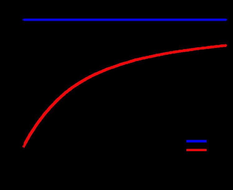
James–Stein estimator - Alchetron, The Free Social Encyclopedia

The James–Stein estimator is a biased estimator of the mean of Gaussian random vectors. It can be shown that the James–Stein estimator dominates the "ordinary" least squares approach, i.e., it has lower mean squared error on average. It is the best-known example of Stein's phenomenon.

Setting

Suppose θ is an unknown parameter vector of length m , and let y be a vector of observations (also of length m ), such that the observations are normally distributed:

y ∼ N ( θ , σ 2 I ) .

We are interested in obtaining an estimate θ ^ = θ ^ ( y ) of θ, based on a single observation vector y.

This is an everyday situation in which a set of parameters is measured, and the measurements are corrupted by independent Gaussian noise. Since the noise has zero mean, it is very reasonable to use the measurements themselves as an estimate of the parameters. This is the approach of the least squares estimator, which is θ ^ L S = y .

As a result, there was considerable shock and disbelief when Stein demonstrated that, in terms of mean squared error E ⁡ [ ∥ θ − θ ^ ∥ 2 ] , this approach is suboptimal. The result became known as Stein's phenomenon.

The James–Stein estimator

If σ 2 is known, the James–Stein estimator is given by

θ ^ J S = ( 1 − ( m − 2 ) σ 2 ∥ y ∥ 2 ) y .

James and Stein showed that the above estimator dominates θ ^ L S for any m ≥ 3 , meaning that the James–Stein estimator always achieves lower mean squared error (MSE) than the maximum likelihood estimator. By definition, this makes the least squares estimator inadmissible when m ≥ 3 .

Notice that if ( m − 2 ) σ 2 < ∥ y ∥ 2 then this estimator simply takes the natural estimator y and shrinks it towards the origin 0. In fact this is not the only direction of shrinkage that works. Let ν be an arbitrary fixed vector of length m . Then there exists an estimator of the James-Stein type that shrinks toward ν, namely

θ ^ J S = ( 1 − ( m − 3 ) σ 2 ∥ y − ν ∥ 2 ) ( y − ν ) + ν , m ≥ 4.

It is interesting to note that the James–Stein estimator dominates the usual estimator for any ν. A natural question to ask is whether the improvement over the usual estimator is independent of the choice of ν. The answer is no. The improvement is small if ∥ θ − ν ∥ is large. Thus to get a very great improvement some knowledge of the location of θ is necessary. Of course this is the quantity we are trying to estimate so we don't have this knowledge a priori. But we may have some guess as to what the mean vector is. This can be considered a disadvantage of the estimator: the choice is not objective as it may depend on the beliefs of the researcher.

Interpretation

Seeing the James–Stein estimator as an empirical Bayes method gives some intuition to this result: One assumes that θ itself is a random variable with prior distribution ∼ N ( 0 , A ) , where A is estimated from the data itself. Estimating A only gives an advantage compared to the maximum-likelihood estimator when the dimension m is large enough; hence it does not work for m ≤ 2 . The James–Stein estimator is a member of a class of Bayesian estimators that dominate the maximum-likelihood estimator.

A consequence of the above discussion is the following counterintuitive result: When three or more unrelated parameters are measured, their total MSE can be reduced by using a combined estimator such as the James–Stein estimator; whereas when each parameter is estimated separately, the least squares (LS) estimator is admissible. A quirky example would be estimating the speed of light, tea consumption in Taiwan, and hog weight in Montana, all together. The James–Stein estimator always improves upon the total MSE, i.e., the sum of the expected errors of each component. Therefore, the total MSE in measuring light speed, tea consumption, and hog weight would improve by using the James–Stein estimator. However, any particular component (such as the speed of light) would improve for some parameter values, and deteriorate for others. Thus, although the James–Stein estimator dominates the LS estimator when three or more parameters are estimated, any single component does not dominate the respective component of the LS estimator.

The conclusion from this hypothetical example is that measurements should be combined if one is interested in minimizing their total MSE. For example, in a telecommunication setting, it is reasonable to combine channel tap measurements in a channel estimation scenario, as the goal is to minimize the total channel estimation error. Conversely, there could be objections to combining channel estimates of different users, since no user would want their channel estimate to deteriorate in order to improve the average network performance.

Improvements

The basic James–Stein estimator has the peculiar property that for small values of ∥ y − ν ∥ , the multiplier on y − ν is actually negative. This can be easily remedied by replacing this multiplier by zero when it is negative. The resulting estimator is called the positive-part James–Stein estimator and is given by

θ ^ J S + = ( 1 − ( m − 3 ) σ 2 ∥ y − ν ∥ 2 ) + ( y − ν ) + ν , m ≥ 4.

This estimator has a smaller risk than the basic James–Stein estimator. It follows that the basic James–Stein estimator is itself inadmissible.

It turns out, however, that the positive-part estimator is also inadmissible. This follows from a general result which requires admissible estimators to be smooth.

Extensions

The James–Stein estimator may seem at first sight to be a result of some peculiarity of the problem setting. In fact, the estimator exemplifies a very wide-ranging effect, namely, the fact that the "ordinary" or least squares estimator is often inadmissible for simultaneous estimation of several parameters. This effect has been called Stein's phenomenon, and has been demonstrated for several different problem settings, some of which are briefly outlined below.

James and Stein demonstrated that the estimator presented above can still be used when the variance σ 2 is unknown, by replacing it with the standard estimator of the variance, σ ^ 2 = 1 n ∑ ( y i − y ¯ ) 2 . The dominance result still holds under the same condition, namely, m > 2 .

The results in this article are for the case when only a single observation vector y is available. For the more general case when n vectors are available, the results are similar:

where y ¯ is the m -length average of the n observations.

The work of James and Stein has been extended to the case of a general measurement covariance matrix, i.e., where measurements may be statistically dependent and may have differing variances. A similar dominating estimator can be constructed, with a suitably generalized dominance condition. This can be used to construct a linear regression technique which outperforms the standard application of the LS estimator.

Stein's result has been extended to a wide class of distributions and loss functions. However, this theory provides only an existence result, in that explicit dominating estimators were not actually exhibited. It is quite difficult to obtain explicit estimators improving upon the usual estimator without specific restrictions on the underlying distributions.

References

James–Stein estimator Wikipedia

(Text) CC BY-SA