Free electron model

Ideas and assumptions

As in the Drude model, valence electrons are assumed to be completely detached from their ions (forming an electron gas). As in an ideal gas, electron-electron interactions are completely neglected. The electrostatic fields in metals are weak because of the screening effect.

The crystal lattice is not explicitly taken into account. A quantum-mechanical justification is given by Bloch's Theorem: an unbound electron moves in a periodic potential as a free electron in vacuum, except for the electron mass m becoming an effective mass m* which may deviate considerably from m (one can even use negative effective mass to describe conduction by electron holes). Effective masses can be derived from band structure computations. While the static lattice does not hinder the motion of the electrons, electrons can be scattered by impurities and by phonons; these two interactions determine electrical and thermal conductivity (superconductivity requires a more refined theory than the free electron model).

According to the Pauli exclusion principle, each phase space element (Δk)³(Δx)³ can be occupied only by two electrons (one per spin quantum number). This restriction of available electron states is taken into account by Fermi–Dirac statistics (see also Fermi gas). Main predictions of the free-electron model are derived by the Sommerfeld expansion of the Fermi–Dirac occupancy for energies around the Fermi level.

Energy and wave function of a free electron

For a free particle the potential is V ( r ) = 0 . The Schrödinger equation for a free particle — in our case an electron — is

− ℏ 2 2 m ∇ 2 Ψ ( r , t ) = i ℏ ∂ ∂ t Ψ ( r , t )

The Schrödinger equation can be solved by separation of variables (see below) to yield a plane wave solution

Ψ ( r , t ) = 1 Ω r e i k ⋅ r − i ω t ,

where k is the wave vector, ω is the frequency, and Ω r is the volume of space where the electron can be found. The electron has kinetic energy

E = ℏ ω = ℏ 2 k 2 2 m

which relates ω and k . For solid state and condensed matter physics, the spatial form

ψ k ( r ) = 1 Ω r e i k ⋅ r

of the plane wave is of major interest. It is the basis of electronic band structure models that are widely used in solid-state physics for model Hamiltonians like the nearly free electron model, the tight binding model and various models that use a muffin-tin approximation. The eigenfunctions of these Hamiltonians are Bloch waves which are modulated plane waves.

Dielectric function of the electron gas

On a scale much larger than the inter atomic distance a solid can be viewed as an aggregate of a negatively charged plasma of the free electron gas and a positively charged background of atomic cores. The background is the rather stiff and massive background of atomic nuclei and core electrons which we will consider to be infinitely massive and fixed in space. The negatively charged plasma is formed by the valence electrons of the free electron model that are uniformly distributed over the interior of the solid. If an oscillating electric field is applied to the solid, the negatively charged plasma tends to move a distance x apart from the positively charged background. As a result, the sample is polarized and there will be an excess charge at the opposite surfaces of the sample. The surface charge density is

ρ s = − n e x

where n is the number density of electrons. This produces a restoring electric field in the sample

E = n e x ϵ 0

The dielectric constant of the sample at a fixed frequency ω is expressed as

ϵ = D ϵ 0 E = 1 + P ϵ 0 E

where D is the electric displacement and P is the polarization density.

The electric field and polarization densities are

E ( t ) = E 0 e − i ω t , P ( t ) = P 0 e − i ω t

and the polarization density with n electron density is

P = − n e x

The force F of the oscillating electric field causes the electrons with charge e and mass m to accelerate with an acceleration a

F = m a = m d 2 x d t 2 = − e E

which, after substitution of E, P and x, yields a harmonic oscillator equation.

After a little algebra the relation between polarization density and electric field can be expressed as

P = − n e 2 m ω 2 E

The frequency dependent dielectric function of the solid is

ϵ ( ω ) = 1 − n e 2 ϵ 0 m ω 2

At a resonance frequency ω p , called the plasma frequency, the dielectric function changes sign from negative to positive and real part of the dielectric function drops to zero.

ω p = n e 2 ϵ 0 m

The plasma frequency represents a plasma oscillation resonance or plasmon. The plasma frequency can be employed as a direct measure of the square root of the density of valence electrons in a solid. Observed values are in reasonable agreement with this theoretical prediction for a large number of materials. Below the plasma frequency, the dielectric function is negative and the field cannot penetrate the sample. Light with angular frequency below the plasma frequency will be totally reflected. Above the plasma frequency the light waves can penetrate the sample.

The Schrödinger equation

For a free particle the potential is V ( r ) = 0 , so the Schrödinger equation for the free electron is

− ℏ 2 2 m ∇ 2 Ψ ( r , t ) = i ℏ ∂ ∂ t Ψ ( r , t )

This is a type of wave equation that has numerous kinds of solutions. One way of solving the equation is splitting it in a time-dependent oscillator equation and a space-dependent wave equation like

i ℏ ∂ ∂ t Ψ ( r , t ) = E Ψ ( r , t )

and

− ℏ 2 2 m ∇ 2 Ψ ( r , t ) = E Ψ ( r , t )

and substituting a product of solutions like

Ψ ( r , t ) = ψ ( r ) e α t

The Schrödinger equation can be split in a time dependent part and a time independent part.Which is derived.

Solution of the time dependent equation

The peculiar time dependent part of the Schrödinger equation is, unlike the Klein–Gordon equation for pions and most of the other well known wave equations, a first order in time differential equation with a 90° out of phase driving mechanism, while most oscillator equations are second order in time differential equations with 180° out of phase driving mechanisms.

The equation that has to be solved is

i ℏ ∂ ∂ t e α t = E e α t .

The complex (imaginary) exponent is proportional to the energy

α = − i E ℏ

The imaginary exponent can be transformed to an angular frequency

E = i ℏ α = ℏ ω

The wave function now has a stationary and an oscillating part

Ψ ( r , t ) = ψ ( r ) e − i ω t

The stationary part is of major importance to the physical properties of the electronic structure of matter.

Solution of the time independent equation

The wave function of free electrons is in general described as the solution of the time independent Schrödinger equation for free electrons

− ℏ 2 2 m ∇ 2 ψ ( r ) = E ψ ( r )

The Laplace operator in Cartesian coordinates is

∇ 2 = ∂ 2 ∂ x 2 + ∂ 2 ∂ y 2 + ∂ 2 ∂ z 2

The wave function can be factorized for the three Cartesian directions

ψ ( r ) = ϕ x ( x ) ϕ y ( y ) ϕ z ( z )

Now the time independent Schrödinger equation can be split in three independent parts for the three different Cartesian directions

− ℏ 2 2 m ∂ 2 ∂ x 2 ϕ x ( x ) = E x ϕ x ( x )

As a solution an exponential function is substituted in the time independent Schrödinger equation

ϕ x ( x ) = N x e κ x

The solution of

∂ 2 ∂ x 2 ϕ x ( x ) = κ 2 N x e κ x = − 2 m ℏ 2 E x N x e κ x

gives the exponent

κ = i k x = i 2 m E x ℏ 2

which yields the wave equation

ψ ( r ) = N x N y N z e i ( k x x + k y y + k z z ) = N k e i k ⋅ r

and the energy

E = ℏ 2 2 m ( k x 2 + k y 2 + k z 2 )

With the normalization

1 = ∫ Ω r | ψ k ( r ) | 2 d r = ∫ Ω r ψ k ∗ ( r ) ψ k ′ ( r ) d r = ∫ Ω r ( N k ∗ e − i k ⋅ r ) ( N k e i k ⋅ r ) d r = N k 2 | Ω r | v o l

and the wave vector magnitude

k = k x 2 + k y 2 + k z 2

we arrive at the plane wave solution with a wave function

ψ k ( r ) = 1 Ω r e i k ⋅ r

for free electrons with a wave vector k and a kinetic energy

E = ℏ 2 k 2 2 m

in which Ω r is the volume of space occupied by the electron.

The traveling plane wave solution

The product of the time independent stationary wave solution and time dependent oscillator solution

Ψ ( r , t ) = ψ ( r ) e − i ω t

gives the traveling plane wave solution

Ψ ( r , t ) = 1 Ω r e i k ⋅ r − i ω t

which is the final solution for the free electron wave function.

Fermi energy

According to the Pauli principle, the electrons in the ground state occupy all the lowest-energy states, up to some Fermi energy E F . Since the energy is given by

E ( k ) = ℏ 2 k 2 2 m ,

this corresponds to occupying all the states with wave vectors | k | < k F , where k F is so-called Fermi wave vector, given by

k F = ( 3 π 2 N e / V ) 1 / 3 ,

where N e is the total number of electrons in the system, and V is the total volume. The Fermi energy is then

In a nearly-free-electron model of a Z -valent metal, one can replace N e with N Z , where N is the total number of metal ions.

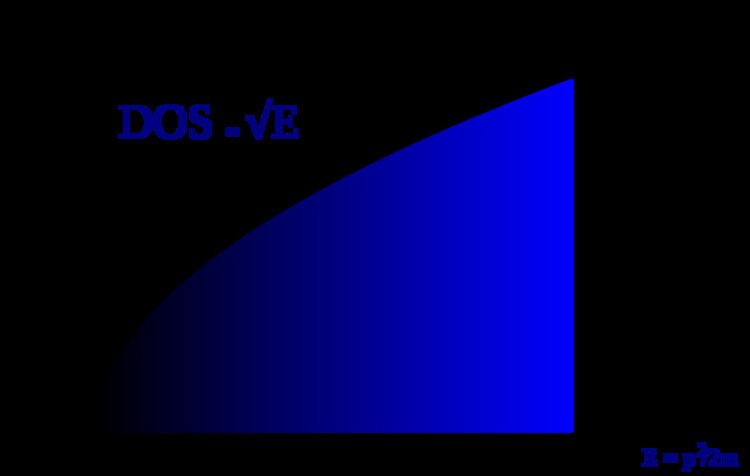
Density of states

The density of states (DOS) corresponds to electrons with a spherically-symmetric parabolic dispersion

E ( k ) = ℏ 2 k 2 2 m ,

with two electrons (one of each spin) per each "quantum" of the phase space, Δ V Δ k = ( 2 π ) 3 . In 3D, this corresponds to

N ( E ) = V 2 π 2 ( 2 m ℏ 2 ) 3 / 2 E ,

where V is the total volume.

Combining these expressions for the Fermi energy and the DOS, one can show that the following relationship holds at the Fermi level:

N ( E F ) = 3 Z N 2 1 E F ,

where Z is the charge of each of the N metal ions in the crystal.