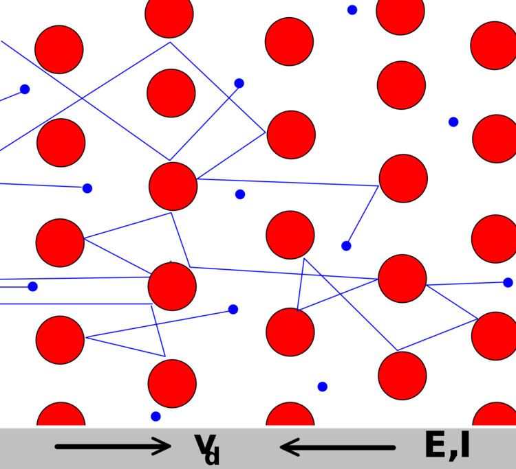
Drude model - Alchetron, The Free Social Encyclopedia

The Drude model of electrical conduction was proposed in 1900 by Paul Drude to explain the transport properties of electrons in materials (especially metals). The model, which is an application of kinetic theory, assumes that the microscopic behavior of electrons in a solid may be treated classically and looks much like a pinball machine, with a sea of constantly jittering electrons bouncing and re-bouncing off heavier, relatively immobile positive ions.

Here t is the time, ⟨p⟩ is the average momentum per electron and q, n, m, and τ are respectively the electron charge, number density, mass, and mean free time between ionic collisions (that is, the mean time an electron has traveled since the last collision, not the average time between collisions). The latter expression is particularly important because it explains in semi-quantitative terms why Ohm's law, one of the most ubiquitous relationships in all of electromagnetism, should be true.

The model was extended in 1905 by Hendrik Antoon Lorentz (and hence is also known as the Drude–Lorentz model) and is a classical model. Later it was supplemented with the results of quantum theory in 1933 by Arnold Sommerfeld and Hans Bethe, leading to the Drude–Sommerfeld model.

Assumptions

The Drude model considers the metal to be formed of a mass of positively charged ions from which a number of "free electrons" were detached. These may be thought to have become delocalized when the valence levels of the atom came in contact with the potential of the other atoms.

The Drude model neglects any long-range interaction between the electron and the ions or between the electrons. The only possible interaction of a free electron with its environment is via instantaneous collisions. The average time between subsequent collisions of such an electron is τ, and the nature of the collision partner of the electron does not matter for the calculations and conclusions of the Drude model.

After a collision event, the velocity (and direction) of the electron only depends on the local temperature distribution and is completely independent of the velocity of the electron before the collision event.

DC field

The simplest analysis of the Drude model assumes that electric field E is both uniform and constant, and that the thermal velocity of electrons is sufficiently high such that they accumulate only an infinitesimal amount of momentum dp between collisions, which occur on average every τ seconds.

Then an electron isolated at time t will on average have been traveling for time τ since its last collision, and consequently will have accumulated momentum

Δ ⟨ p ⟩ = q E τ .

During its last collision, this electron will have been just as likely to have bounced forward as backward, so all prior contributions to the electron's momentum may be ignored, resulting in the expression

⟨ p ⟩ = q E τ .

Substituting the relations

⟨ p ⟩ = m ⟨ v ⟩ , J = n q ⟨ v ⟩ ,

results in the formulation of Ohm's law mentioned above:

J = ( n q 2 τ m ) E .

Time-varying analysis

The dynamics may also be described by introducing an effective drag force. At time t = t₀ + dt the average electron's momentum will be

⟨ p ( t 0 + d t ) ⟩ = ( 1 − d t τ ) ( ⟨ p ( t 0 ) ⟩ + q E d t ) ,

because, on average, a fraction of 1 − dt/τ of the electrons will not have experienced another collision, and the ones that have will contribute to the total momentum to only a negligible order.

With a bit of algebra and dropping terms of order dt², this results in the differential equation

d d t ⟨ p ( t ) ⟩ = q E − ⟨ p ( t ) ⟩ τ ,

where ⟨p⟩ denotes average momentum and q the charge of the electrons. This, which is an inhomogeneous differential equation, may be solved to obtain the general solution of

⟨ p ( t ) ⟩ = q τ E ( 1 − e − t / τ ) + ⟨ p ( 0 ) ⟩ e − t / τ

for p(t). The steady state solution (d ⟨p⟩/dt = 0) is then

⟨ p ⟩ = q τ E .

As above, average momentum may be related to average velocity and this in turn may be related to current density,

⟨ p ⟩ = m ⟨ v ⟩ , J = n q ⟨ v ⟩ ,

and the material can be shown to satisfy Ohm's law with a DC-conductivity σ₀:

J = ( n q 2 τ m ) E .

The Drude model can also predict the current as a response to a time-dependent electric field with an angular frequency ω, in which case

σ ( ω ) = σ 0 1 + i ω τ = σ 0 1 + ω 2 τ 2 − i ω τ σ 0 1 + ω 2 τ 2 .

Here it is assumed that

E ( t ) = ℜ ( E 0 e i ω t ) ; J ( t ) = ℜ ( σ ( ω ) E 0 e i ω t ) .

In other conventions, i is replaced by −i in all equations. The imaginary part indicates that the current lags behind the electrical field, which happens because the electrons need roughly a time τ to accelerate in response to a change in the electrical field. Here the Drude model is applied to electrons; it can be applied both to electrons and holes; i.e., positive charge carriers in semiconductors. The curves for σ(ω) are shown in the graph.

Drude response in real materials

The characteristic behavior of a Drude metal in the time or frequency domain, i.e. exponential relaxation with time constant τ or the frequency dependence for σ(ω) stated above, is called Drude response. In a conventional, simple, real metal (e.g. sodium, silver, or gold at room temperature) such behavior is not found experimentally, because the characteristic frequency τ⁻¹ is in the infrared frequency range, where other features that are not considered in the Drude model (such as band structure) play an important role. But for certain other materials with metallic properties, frequency-dependent conductivity was found that closely follows the simple Drude prediction for σ(ω). These are materials where the relaxation rate τ⁻¹ is at much lower frequencies. This is the case for certain doped semiconductor single crystals, high-mobility two-dimensional electron gases, and heavy-fermion metals.

Accuracy of the model

Historically, the Drude formula was first derived in an incorrect way, namely by assuming that the charge carriers form an ideal gas. It is now known that they follow Fermi–Dirac distribution and have appreciable interactions, but amazingly, the result turns out to be the same as the Drude model because, as Lev Landau derived in 1957, a gas of interacting particles can be described by a system of almost non-interacting 'quasiparticles' that, in the case of electrons in a metal, can be well modelled by the Drude equation.

This simple classical Drude model provides a very good explanation of DC and AC conductivity in metals, the Hall effect, and thermal conductivity (due to electrons) in metals near room temperature. The model also explains the Wiedemann–Franz law of 1853. However, it greatly overestimates the electronic heat capacities of metals. In reality, metals and insulators have roughly the same heat capacity at room temperature. The model can be applied to positive (hole) charge carriers, as demonstrated by the Hall effect.

One note of trivia surrounding the theory is that in his original paper Drude made a conceptual error, estimating electrical conductivity to in fact be only half of what it classically should have been.

References

Drude model Wikipedia

(Text) CC BY-SA