
 | ||
Fracture mechanics is the field of mechanics concerned with the study of the propagation of cracks in materials. It uses methods of analytical solid mechanics to calculate the driving force on a crack and those of experimental solid mechanics to characterize the material's resistance to fracture.
Contents
- Motivation
- Griffiths criterion
- Irwins modification
- Stress intensity factor
- Strain energy release
- Crack tip plastic zone
- Limitations
- Elasticplastic fracture mechanics
- CTOD
- R curve
- J integral
- Cohesive zone models
- Transition flaw size
- Crack tip constraint under large scale yielding
- J Q Theory
- T term effects
- Engineering applications
- Irwins modifications
- Elasticity and plasticity
- Applications of fracture mechanics
- References
In modern materials science, fracture mechanics is an important tool used to improve the performance of mechanical components. It applies the physics of stress and strain behavior of materials, in particular the theories of elasticity and plasticity, to the microscopic crystallographic defects found in real materials in order to predict the macroscopic mechanical behavior of those bodies. Fractography is widely used with fracture mechanics to understand the causes of failures and also verify the theoretical failure predictions with real life failures. The prediction of crack growth is at the heart of the damage tolerance mechanical design discipline.
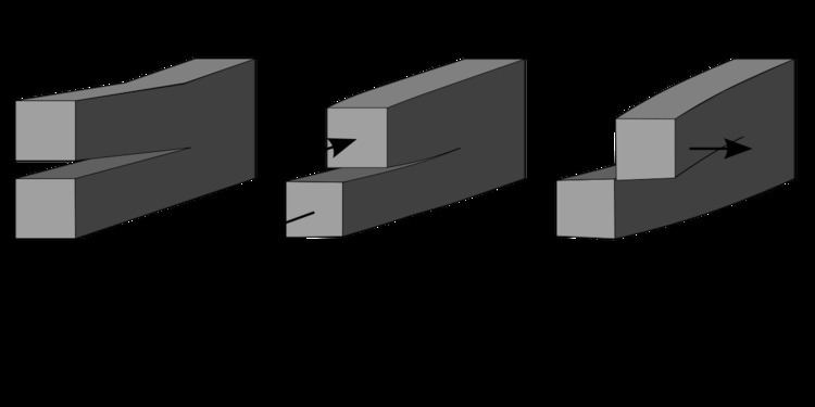
There are three ways of applying a force to enable a crack to propagate:
Motivation
The processes of material manufacture, processing, machining, and forming may introduce flaws in a finished mechanical component. Arising from the manufacturing process, interior and surface flaws are found in all metal structures. Not all such flaws are unstable under service conditions. Fracture mechanics is the analysis of flaws to discover those that are safe (that is, do not grow) and those that are liable to propagate as cracks and so cause failure of the flawed structure. Despite these inherent flaws, it is possible to achieve through damage tolerance analysis the safe operation of a structure. Fracture mechanics as a subject for critical study has barely been around for a century and thus is relatively new.
Fracture mechanics should attempt to provide quantitative answers to the following questions:
- What is the strength of the component as a function of crack size?
- What crack size can be tolerated under service loading, i.e. what is the maximum permissible crack size?
- How long does it take for a crack to grow from a certain initial size, for example the minimum detectable crack size, to the maximum permissible crack size?
- What is the service life of a structure when a certain pre-existing flaw size (e.g. a manufacturing defect) is assumed to exist?
- During the period available for crack detection how often should the structure be inspected for cracks?
Griffith's criterion
Fracture mechanics was developed during World War I by English aeronautical engineer, A. A. Griffith, to explain the failure of brittle materials. Griffith's work was motivated by two contradictory facts:
A theory was needed to reconcile these conflicting observations. Also, experiments on glass fibers that Griffith himself conducted suggested that the fracture stress increases as the fiber diameter decreases. Hence the uniaxial tensile strength, which had been used extensively to predict material failure before Griffith, could not be a specimen-independent material property. Griffith suggested that the low fracture strength observed in experiments, as well as the size-dependence of strength, was due to the presence of microscopic flaws in the bulk material.
To verify the flaw hypothesis, Griffith introduced an artificial flaw in his experimental glass specimens. The artificial flaw was in the form of a surface crack which was much larger than other flaws in a specimen. The experiments showed that the product of the square root of the flaw length (a) and the stress at fracture (σf) was nearly constant, which is expressed by the equation:
An explanation of this relation in terms of linear elasticity theory is problematic. Linear elasticity theory predicts that stress (and hence the strain) at the tip of a sharp flaw in a linear elastic material is infinite. To avoid that problem, Griffith developed a thermodynamic approach to explain the relation that he observed.
The growth of a crack, the extension of the surfaces on either side of the crack, requires an increase in the surface energy. Griffith found an expression for the constant C in terms of the surface energy of the crack by solving the elasticity problem of a finite crack in an elastic plate. Briefly, the approach was:
where E is the Young's modulus of the material and γ is the surface energy density of the material. Assuming E = 62 GPa and γ = 1 J/m2 gives excellent agreement of Griffith's predicted fracture stress with experimental results for glass.
Irwin's modification
Griffith's work was largely ignored by the engineering community until the early 1950s. The reasons for this appear to be (a) in the actual structural materials the level of energy needed to cause fracture is orders of magnitude higher than the corresponding surface energy, and (b) in structural materials there are always some inelastic deformations around the crack front that would make the assumption of linear elastic medium with infinite stresses at the crack tip highly unrealistic.
Griffith's theory provides excellent agreement with experimental data for brittle materials such as glass. For ductile materials such as steel, although the relation
In ductile materials (and even in materials that appear to be brittle), a plastic zone develops at the tip of the crack. As the applied load increases, the plastic zone increases in size until the crack grows and the elastically strained material behind the crack tip unloads. The plastic loading and unloading cycle near the crack tip leads to the dissipation of energy as heat. Hence, a dissipative term has to be added to the energy balance relation devised by Griffith for brittle materials. In physical terms, additional energy is needed for crack growth in ductile materials as compared to brittle materials.
Irwin's strategy was to partition the energy into two parts:
where γ is the surface energy and Gp is the plastic dissipation (and dissipation from other sources) per unit area of crack growth.
The modified version of Griffith's energy criterion can then be written as
For brittle materials such as glass, the surface energy term dominates and
Stress intensity factor
Another significant achievement of Irwin and his colleagues was to find a method of calculating the amount of energy available for fracture in terms of the asymptotic stress and displacement fields around a crack front in a linear elastic solid. This asymptotic expression for the stress field around a crack tip is
where σij are the Cauchy stresses, r is the distance from the crack tip, θ is the angle with respect to the plane of the crack, and fij are functions that depend on the crack geometry and loading conditions. Irwin called the quantity K the stress intensity factor. Since the quantity fij is dimensionless, the stress intensity factor can be expressed in units of
When a rigid line inclusion is considered, a similar asymptotic expression for the stress fields is obtained.
Strain energy release
Irwin was the first to observe that if the size of the plastic zone around a crack is small compared to the size of the crack, the energy required to grow the crack will not be critically dependent on the state of stress (the plastic zone) at the crack tip. In other words, a purely elastic solution may be used to calculate the amount of energy available for fracture.
The energy release rate for crack growth or strain energy release rate may then be calculated as the change in elastic strain energy per unit area of crack growth, i.e.,
where U is the elastic energy of the system and a is the crack length. Either the load P or the displacement u are constant while evaluating the above expressions.
Irwin showed that for a mode I crack (opening mode) the strain energy release rate and the stress intensity factor are related by:
where E is the Young's modulus, ν is Poisson's ratio, and KI is the stress intensity factor in mode I. Irwin also showed that the strain energy release rate of a planar crack in a linear elastic body can be expressed in terms of the mode I, mode II (sliding mode), and mode III (tearing mode) stress intensity factors for the most general loading conditions.
Next, Irwin adopted the additional assumption that the size and shape of the energy dissipation zone remains approximately constant during brittle fracture. This assumption suggests that the energy needed to create a unit fracture surface is a constant that depends only on the material. This new material property was given the name fracture toughness and designated GIc. Today, it is the critical stress intensity factor KIc, found in the plane strain condition, which is accepted as the defining property in linear elastic fracture mechanics.
Crack tip plastic zone
In theory the stress at the crack tip where the radius is nearly zero, would tend to infinity. This would be considered a stress singularity, which is not possible in real-world applications. In actuality, the stress concentration at the tip of a crack within real materials has been found to have a finite value but larger than the nominal stress applied to the specimen. An equation giving the stresses near a crack tip is given below:
The stress near the crack tip,
Models of ideal materials have shown that this zone of plasticity is centered at the crack tip. This equation gives the approximate ideal radius of the plastic zone deformation beyond the crack tip, which is useful to many structural scientists because it gives a good estimate of how the material behaves when subjected to stress. In the above equation, the parameters of the stress intensity factor and indicator of material toughness,
The same process as described above for a single event loading also applies and to cyclic loading. If a crack is present in a specimen that undergoes cyclic loading, the specimen will plastically deform at the crack tip and delay the crack growth. In the event of an overload or excursion, this model changes slightly to accommodate the sudden increase in stress from that which the material previously experienced. At a sufficiently high load (overload), the crack grows out of the plastic zone that contained it and leaves behind the pocket of the original plastic deformation. Now, assuming that the overload stress is not sufficiently high as to completely fracture the specimen, the crack will undergo further plastic deformation around the new crack tip, enlarging the zone of residual plastic stresses. This process further toughens and prolongs the life of the material because the new plastic zone is larger than what it would be under the usual stress conditions. This allows the material to undergo more cycles of loading. This idea can be illustrated further by the graph of Aluminum with a center crack undergoing overloading events.
Limitations
But a problem arose for the NRL researchers because naval materials, e.g., ship-plate steel, are not perfectly elastic but undergo significant plastic deformation at the tip of a crack. One basic assumption in Irwin's linear elastic fracture mechanics is small scale yielding, the condition that the size of the plastic zone is small compared to the crack length. However, this assumption is quite restrictive for certain types of failure in structural steels though such steels can be prone to brittle fracture, which has led to a number of catastrophic failures.
Linear-elastic fracture mechanics is of limited practical use for structural steels and Fracture toughness testing can be expensive.
Elastic–plastic fracture mechanics
Most engineering materials show some nonlinear elastic and inelastic behavior under operating conditions that involve large loads. In such materials the assumptions of linear elastic fracture mechanics may not hold, that is,
Therefore, a more general theory of crack growth is needed for elastic-plastic materials that can account for:
CTOD
Historically, the first parameter for the determination of fracture toughness in the elasto-plastic region was the crack tip opening displacement (CTOD) or "opening at the apex of the crack" indicated. This parameter was determined by Wells during the studies of structural steels which, due to the high toughness could not be characterized with the linear elastic fracture mechanics model. He noted that, before the fracture happened, the walls of the crack were leaving and that the crack tip, after fracture, ranged from acute to rounded off due to plastic deformation. In addition, the rounding of the crack tip was more pronounced in steels with superior toughness.
There are a number of alternative definitions of CTOD. The two most common definitions, CTOD is the displacement at the original crack tip and the 90 degree intercept. The latter definition was suggested by Rice and is commonly used to infer CTOD in finite element models of such. Note that these two definitions are equivalent if the crack tip blunts in a semicircle.
Most laboratory measurements of CTOD have been made on edge-cracked specimens loaded in three-point bending. Early experiments used a flat paddle-shaped gage that was inserted into the crack; as the crack opened, the paddle gage rotated, and an electronic signal was sent to an x-y plotter. This method was inaccurate, however, because it was difficult to reach the crack tip with the paddle gage. Today, the displacement V at the crack mouth is measured, and the CTOD is inferred by assuming the specimen halves are rigid and rotate about a hinge point (the crack tip).
R-curve
An early attempt in the direction of elastic-plastic fracture mechanics was Irwin's crack extension resistance curve, Crack growth resistance curve or R-curve. This curve acknowledges the fact that the resistance to fracture increases with growing crack size in elastic-plastic materials. The R-curve is a plot of the total energy dissipation rate as a function of the crack size and can be used to examine the processes of slow stable crack growth and unstable fracture. However, the R-curve was not widely used in applications until the early 1970s. The main reasons appear to be that the R-curve depends on the geometry of the specimen and the crack driving force may be difficult to calculate.
J-integral
In the mid-1960s James R. Rice (then at Brown University) and G. P. Cherepanov independently developed a new toughness measure to describe the case where there is sufficient crack-tip deformation that the part no longer obeys the linear-elastic approximation. Rice's analysis, which assumes non-linear elastic (or monotonic deformation theory plastic) deformation ahead of the crack tip, is designated the J-integral. This analysis is limited to situations where plastic deformation at the crack tip does not extend to the furthest edge of the loaded part. It also demands that the assumed non-linear elastic behavior of the material is a reasonable approximation in shape and magnitude to the real material's load response. The elastic-plastic failure parameter is designated JIc and is conventionally converted to KIc using Equation (3.1) of the Appendix to this article. Also note that the J integral approach reduces to the Griffith theory for linear-elastic behavior.
The mathematical definition of J-integral is as follows:
where
Cohesive zone models
When a significant region around a crack tip has undergone plastic deformation, other approaches can be used to determine the possibility of further crack extension and the direction of crack growth and branching. A simple technique that is easily incorporated into numerical calculations is the cohesive zone model method which is based on concepts proposed independently by Barenblatt and Dugdale in the early 1960s. The relationship between the Dugdale-Barenblatt models and Griffith's theory was first discussed by Willis in 1967. The equivalence of the two approaches in the context of brittle fracture was shown by Rice in 1968. Interest in cohesive zone modeling of fracture has been reignited since 2000 following the pioneering work on dynamic fracture by Xu and Needleman, and Camacho and Ortiz.
Transition flaw size
Let a material have a yield strength
Crack tip constraint under large scale yielding
Under small-scale yielding conditions, a single parameter (e.g., K, J, or CTOD) characterizes crack tip conditions and can be used as a geometry-independent fracture criterion. Single-parameter fracture mechanics breaks down in the presence of excessive plasticity, and when the fracture toughness depends on the size and geometry of the test specimen. The theories used for large scale yielding is not very standardized. The following theories and approaches are commonly used among researchers in this field.
J-Q Theory
By using FEM, one can establish a parameter Q to modify the stress field for a better solution when the plastic zone is growing. The new stress field is:
The J-Q-M theory includes another parameter, the mismatch parameter, which is used for welds to make up for the change in toughness of the weld metal (WM), base metal (BM) and heat affected zone (HAZ). This value is interpreted to the formula in a similar way as the Q-parameter, and the two are usually assumed to be independent of each other.
T-term effects
As an alternative to J-Q theory, a parameter T can be used. This only changes the normal stress in the x-direction (and the z-direction in the case of plane strain). T does not require the use of FEM, but is derived from constraint. It can be argued that T is limited to LEFM, but as the plastic zone change due to T never reaches the actual crack surface (except on the tip), its validity holds true not only under small scale yielding. The parameter T also significantly influences on the fracture initiation in brittle materials using maximum tangential strain fracture criterion, as found by the researchers at Texas A&M University. It is found that both parameter T and Poisson's ratio of the material play important roles in prediction of the crack propagation angle and the mixed mode fracture toughness of the materials.
Engineering applications
The following information is needed for a fracture mechanics prediction of failure:
Usually not all of this information is available and conservative assumptions have to be made.
Occasionally post-mortem fracture-mechanics analyses are carried out. In the absence of an extreme overload, the causes are either insufficient toughness (KIc) or an excessively large crack that was not detected during routine inspection.
Griffith's criterion
For the simple case of a thin rectangular plate with a crack perpendicular to the load Griffith’s theory becomes:
where
However, we also have that:
If
Irwin's modifications
Eventually a modification of Griffith’s solids theory emerged from this work; a term called stress intensity replaced strain energy release rate and a term called fracture toughness replaced surface weakness energy. Both of these terms are simply related to the energy terms that Griffith used:
and
where KI is the stress intensity, Kc the fracture toughness, and
Fracture occurs when
We must note that the expression for
where Y is a function of the crack length and width of sheet given by:
for a sheet of finite width W containing a through-thickness crack of length 2a, or
for a sheet of finite width W containing a through-thickness edge crack of length a
Elasticity and plasticity
Since engineers became accustomed to using KIc to characterise fracture toughness, a relation has been used to reduce JIc to it:
The remainder of the mathematics employed in this approach is interesting, but is probably better summarised in external pages due to its complex nature.
Applications of fracture mechanics
The design process for a component consists of choosing the appropriate geometry, the necessary material strength, the temperature of usage and method of structural analysis (Testing and FEM analysis), so as to ensure that it does not fail under load. The methodologies followed in design criteria traditionally invole the selection of materials based on standard data and as per the loading conditions proportioning the geometry of the components on basis of an analysis. This method is not applicable for some new innovation like usage of new material in design. Another method followed is that as per the loading conditions, static analysis is done for the structure taking into account the forces acting on each component, material strength and geometry. The material strength is chosen keeping in mind the factor of safety, i.e. the component is designed to withstand an ultimate load (where it fails) greater than the load under which it will operate. A general assumption in the design criteria are is the lack of discontinuities, no defects or cracks in the material, and even in the presence of such discontinuities the material is assumed to have sufficient ductility to yield locally so to allow a redistribution of stress at those discontinuities. However, the investigation of failed components demonstrate such assumptions to often be incorrect and that crack growth started because of such discontinuities.
Fracture mechanics follows one of two design principles: either fail-safe or safe-life. In fail-safe mode, even if a component fails, the entire structure is not at risk due to load path redundancy; this may lead to complicated and heavy structures. The safe-life principle dictates that throughout the life of the structure, no component of the structure may fail. This may lead to single load paths, but requires a more detailed analysis that employs fracture mechanics to ensure no failure during the defined lifetime. Fracture mechanics estimates the maximum length of crack that a material can withstand before it fails using an analysis that takes into consideration the overall dimensions of the structure, the stresses where crack initiation takes place, notch toughness of the material (a measure of the ability of a material to absorb energy before the crack extends) Kc, the behavior of materials under the action of stresses giving a stress intensity factor (K), fatigue crack growth, and stress corrosion crack growth. As with basic solid mechanics analysis, the stresses in the component should be lower than the yield stress. By analogy, the stress intensity factor, K, should be less than the critical stress intensity factor Kc. Ultimately, a safe-life analysis leads to a prediction of the lifetime of a component with an approriate degree of confidence. The main conclusions of fracture mechanics analysis to a design are the proper material selection, effect of defects, failure analysis, and development of time schedules to monitor components for cracks. Fracture analysis includes the usage of mathematical models such as linear elastic fracture mechanics (LEFM), crack opening displacement (COD) and J-integral approaches by using finite element analysis (FEM).
The relationship used for estimating stress intensity factor is
where c a constant that depends on crack and specimen dimensions, σ the applied stress, and a the crack length.
The above relation is very general and as per the shape of the crack, relations available in standard references are to be used, standard shapes of cracks approximating actual cracks can be used.
For a given material the value of K is dependent on the applied stresses and flaw size. The flaw sized that will cause crack extension decreases as the stress increases. Thus by chosing two of the three parameters (K, a and σ) the design is constrained by the remaining unknown. Even so, there are other parameters that affect the life of a component, such as working temperature, repeated loading (fatigue), residual stress, and stress concentration effects. If a material is chosen, that will fix the value of the critical notch toughness Kc value. If a value of the minimum size crack length, a, is also selected, that allows the solution for σ the stress near the crack below which the component must be kept. The latter allows the sizing of the component.
Designers try to decrease the defects in the component arising in manufacturing processes by following good fabrication processes and inspection, and estimate notch-toughness values (Kc) of materials using methods like charpy V-notch impact test, or drop weight tests. In many investigations it was proved that the material failed at a K value very much lower than the critical stress intensity factor because of defects in the material or micro cracks. Analysis proved that for any component there are two phases for crack development, i.e. crack initiation and second phase crack growth until failure. Of the two, the first phase covers a larger percentage of fatigue life, and under very large high cycle loading conditions the second phase is very short.
The factor (K/σ)² is used for the initial design of a component because it estimates crack size. But how large this factor has to be is decided by considering type of the structure, frequency of inspection, accessibility to inspection, design life of the structure, consequences of failure, probability of over-load, methods of fabrication, required quality, material cost in addition to the results obtained by fracture mechanics analysis.