Fibonacci heap

Structure

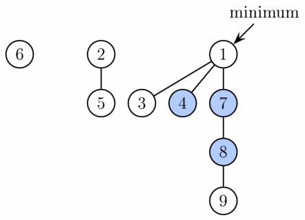
A Fibonacci heap is a collection of trees satisfying the minimum-heap property, that is, the key of a child is always greater than or equal to the key of the parent. This implies that the minimum key is always at the root of one of the trees. Compared with binomial heaps, the structure of a Fibonacci heap is more flexible. The trees do not have a prescribed shape and in the extreme case the heap can have every element in a separate tree. This flexibility allows some operations to be executed in a lazy manner, postponing the work for later operations. For example, merging heaps is done simply by concatenating the two lists of trees, and operation decrease key sometimes cuts a node from its parent and forms a new tree.

However, at some point order needs to be introduced to the heap to achieve the desired running time. In particular, degrees of nodes (here degree means the number of children) are kept quite low: every node has degree at most O(log n) and the size of a subtree rooted in a node of degree k is at least F_k+2, where F_k is the kth Fibonacci number. This is achieved by the rule that we can cut at most one child of each non-root node. When a second child is cut, the node itself needs to be cut from its parent and becomes the root of a new tree (see Proof of degree bounds, below). The number of trees is decreased in the operation delete minimum, where trees are linked together.

As a result of a relaxed structure, some operations can take a long time while others are done very quickly. For the amortized running time analysis we use the potential method, in that we pretend that very fast operations take a little bit longer than they actually do. This additional time is then later combined and subtracted from the actual running time of slow operations. The amount of time saved for later use is measured at any given moment by a potential function. The potential of a Fibonacci heap is given by

where t is the number of trees in the Fibonacci heap, and m is the number of marked nodes. A node is marked if at least one of its children was cut since this node was made a child of another node (all roots are unmarked). The amortized time for an operation is given by the sum of the actual time and c times the difference in potential, where c is a constant (chosen to match the constant factors in the O notation for the actual time).

Thus, the root of each tree in a heap has one unit of time stored. This unit of time can be used later to link this tree with another tree at amortized time 0. Also, each marked node has two units of time stored. One can be used to cut the node from its parent. If this happens, the node becomes a root and the second unit of time will remain stored in it as in any other root.

Implementation of operations

To allow fast deletion and concatenation, the roots of all trees are linked using a circular, doubly linked list. The children of each node are also linked using such a list. For each node, we maintain its number of children and whether the node is marked. Moreover, we maintain a pointer to the root containing the minimum key.

Operation find minimum is now trivial because we keep the pointer to the node containing it. It does not change the potential of the heap, therefore both actual and amortized cost are constant.

As mentioned above, merge is implemented simply by concatenating the lists of tree roots of the two heaps. This can be done in constant time and the potential does not change, leading again to constant amortized time.

Operation insert works by creating a new heap with one element and doing merge. This takes constant time, and the potential increases by one, because the number of trees increases. The amortized cost is thus still constant.

Operation extract minimum (same as delete minimum) operates in three phases. First we take the root containing the minimum element and remove it. Its children will become roots of new trees. If the number of children was d, it takes time O(d) to process all new roots and the potential increases by d−1. Therefore, the amortized running time of this phase is O(d) = O(log n).

However to complete the extract minimum operation, we need to update the pointer to the root with minimum key. Unfortunately there may be up to n roots we need to check. In the second phase we therefore decrease the number of roots by successively linking together roots of the same degree. When two roots u and v have the same degree, we make one of them a child of the other so that the one with the smaller key remains the root. Its degree will increase by one. This is repeated until every root has a different degree. To find trees of the same degree efficiently we use an array of length O(log n) in which we keep a pointer to one root of each degree. When a second root is found of the same degree, the two are linked and the array is updated. The actual running time is O(log n + m) where m is the number of roots at the beginning of the second phase. At the end we will have at most O(log n) roots (because each has a different degree). Therefore, the difference in the potential function from before this phase to after it is: O(log n) − m, and the amortized running time is then at most O(log n + m) + c(O(log n) − m). With a sufficiently large choice of c, this simplifies to O(log n).

In the third phase we check each of the remaining roots and find the minimum. This takes O(log n) time and the potential does not change. The overall amortized running time of extract minimum is therefore O(log n).

Operation decrease key will take the node, decrease the key and if the heap property becomes violated (the new key is smaller than the key of the parent), the node is cut from its parent. If the parent is not a root, it is marked. If it has been marked already, it is cut as well and its parent is marked. We continue upwards until we reach either the root or an unmarked node. Now we set the minimum pointer to the decreased value if it is the new minimum. In the process we create some number, say k, of new trees. Each of these new trees except possibly the first one was marked originally but as a root it will become unmarked. One node can become marked. Therefore, the number of marked nodes changes by −(k − 1) + 1 = − k + 2. Combining these 2 changes, the potential changes by 2(−k + 2) + k = −k + 4. The actual time to perform the cutting was O(k), therefore (again with a sufficiently large choice of c) the amortized running time is constant.

Finally, operation delete can be implemented simply by decreasing the key of the element to be deleted to minus infinity, thus turning it into the minimum of the whole heap. Then we call extract minimum to remove it. The amortized running time of this operation is O(log n).

Proof of degree bounds

The amortized performance of a Fibonacci heap depends on the degree (number of children) of any tree root being O(log n), where n is the size of the heap. Here we show that the size of the (sub)tree rooted at any node x of degree d in the heap must have size at least F_d+2, where F_k is the kth Fibonacci number. The degree bound follows from this and the fact (easily proved by induction) that F d + 2 ≥ φ d for all integers d ≥ 0 , where φ = ( 1 + 5 ) / 2 ≐ 1.618 . (We then have n ≥ F d + 2 ≥ φ d , and taking the log to base φ of both sides gives d ≤ log φ ⁡ n as required.)

Consider any node x somewhere in the heap (x need not be the root of one of the main trees). Define size(x) to be the size of the tree rooted at x (the number of descendants of x, including x itself). We prove by induction on the height of x (the length of a longest simple path from x to a descendant leaf), that size(x) ≥ F_d+2, where d is the degree of x.

Base case: If x has height 0, then d = 0, and size(x) = 1 = F₂.

Inductive case: Suppose x has positive height and degree d>0. Let y₁, y₂, ..., y_d be the children of x, indexed in order of the times they were most recently made children of x (y₁ being the earliest and y_d the latest), and let c₁, c₂, ..., c_d be their respective degrees. We claim that c_i ≥ i-2 for each i with 2≤i≤d: Just before y_i was made a child of x, y₁,...,y_i−1 were already children of x, and so x had degree at least i−1 at that time. Since trees are combined only when the degrees of their roots are equal, it must have been that y_i also had degree at least i-1 at the time it became a child of x. From that time to the present, y_i can only have lost at most one child (as guaranteed by the marking process), and so its current degree c_i is at least i−2. This proves the claim.

Since the heights of all the y_i are strictly less than that of x, we can apply the inductive hypothesis to them to get size(y_i) ≥ F_ci+2 ≥ F_(i−2)+2 = F_i. The nodes x and y₁ each contribute at least 1 to size(x), and so we have

size ( x ) ≥ 2 + ∑ i = 2 d size ( y i ) ≥ 2 + ∑ i = 2 d F i = 1 + ∑ i = 0 d F i .

A routine induction proves that 1 + ∑ i = 0 d F i = F d + 2 for any d ≥ 0 , which gives the desired lower bound on size(x).

Worst case

Although Fibonacci heaps look very efficient, they have the following two drawbacks (as mentioned in the paper "The Pairing Heap: A new form of Self Adjusting Heap"): "They are complicated when it comes to coding them. Also they are not as efficient in practice when compared with the theoretically less efficient forms of heaps, since in their simplest version they require storage and manipulation of four pointers per node, compared to the two or three pointers per node needed for other structures ". These other structures are referred to Binary heap, Binomial heap, Pairing Heap, Brodal Heap and Rank Pairing Heap.

Although the total running time of a sequence of operations starting with an empty structure is bounded by the bounds given above, some (very few) operations in the sequence can take very long to complete (in particular delete and delete minimum have linear running time in the worst case). For this reason Fibonacci heaps and other amortized data structures may not be appropriate for real-time systems. It is possible to create a data structure which has the same worst-case performance as the Fibonacci heap has amortized performance. One such structure, the Brodal queue, is, in the words of the creator, "quite complicated" and "[not] applicable in practice." Created in 2012, the strict Fibonacci heap is a simpler (compared to Brodal's) structure with the same worst-case bounds. It is unknown whether the strict Fibonacci heap is efficient in practice. The run-relaxed heaps of Driscoll et al. give good worst-case performance for all Fibonacci heap operations except merge.

Summary of running times

In the following time complexities O(f) is an asymptotic upper bound and Θ(f) is an asymptotically tight bound (see Big O notation). Function names assume a min-heap.

Practical considerations

Fibonacci heaps have a reputation for being slow in practice due to large memory consumption per node and high constant factors on all operations. Recent experimental results suggest that Fibonacci heaps are more efficient in practice than most of its later derivatives, including quake heaps, violation heaps, strict Fibonacci heaps, rank pairing heaps, but less efficient than either pairing heaps or array-based heaps.