Fabry–Pérot interferometer

Basic description

The heart of the Fabry–Pérot interferometer is a pair of partially reflective glass optical flats spaced micrometers to centimeters apart, with the reflective surfaces facing each other. (Alternatively, a Fabry–Pérot etalon uses a single plate with two parallel reflecting surfaces.) The flats in an interferometer are often made in a wedge shape to prevent the rear surfaces from producing interference fringes; the rear surfaces often also have an anti-reflective coating.

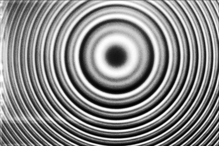
In a typical system, illumination is provided by a diffuse source set at the focal plane of a collimating lens. A focusing lens after the pair of flats would produce an inverted image of the source if the flats were not present; all light emitted from a point on the source is focused to a single point in the system's image plane. In the accompanying illustration, only one ray emitted from point A on the source is traced. As the ray passes through the paired flats, it is multiply reflected to produce multiple transmitted rays which are collected by the focusing lens and brought to point A' on the screen. The complete interference pattern takes the appearance of a set of concentric rings. The sharpness of the rings depends on the reflectivity of the flats. If the reflectivity is high, resulting in a high Q factor, monochromatic light produces a set of narrow bright rings against a dark background. A Fabry–Pérot interferometer with high Q is said to have high finesse.

Applications

Telecommunications networks employing wavelength division multiplexing have add-drop multiplexers with banks of miniature tuned fused silica or diamond etalons. These are small iridescent cubes about 2 mm on a side, mounted in small high-precision racks. The materials are chosen to maintain stable mirror-to-mirror distances, and to keep stable frequencies even when the temperature varies. Diamond is preferred because it has greater heat conduction and still has a low coefficient of expansion. In 2005, some telecommunications equipment companies began using solid etalons that are themselves optical fibers. This eliminates most mounting, alignment and cooling difficulties.

Dichroic filters are made by depositing a series of etalonic layers on an optical surface by vapor deposition. These optical filters usually have more exact reflective and pass bands than absorptive filters. When properly designed, they run cooler than absorptive filters because they can reflect unwanted wavelengths. Dichroic filters are widely used in optical equipment such as light sources, cameras, astronomical equipment, and laser systems.

Optical wavemeters and some optical spectrum analyzers use Fabry–Pérot interferometers with different free spectral ranges to determine the wavelength of light with great precision.

Laser resonators are often described as Fabry–Pérot resonators, although for many types of laser the reflectivity of one mirror is close to 100%, making it more similar to a Gires–Tournois interferometer. Semiconductor diode lasers sometimes use a true Fabry–Pérot geometry, due to the difficulty of coating the end facets of the chip. Quantum cascade lasers often employ Fabry-Pérot cavities to sustain lasing without the need for any facet coatings, due to the high gain of the active region.

Etalons are often placed inside the laser resonator when constructing single-mode lasers. Without an etalon, a laser will generally produce light over a wavelength range corresponding to a number of cavity modes, which are similar to Fabry–Pérot modes. Inserting an etalon into the laser cavity, with well-chosen finesse and free-spectral range, can suppress all cavity modes except for one, thus changing the operation of the laser from multi-mode to single-mode.

Fabry–Pérot etalons can be used to prolong the interaction length in laser absorption spectrometry, particularly cavity ring-down, techniques.

A Fabry–Pérot etalon can be used to make a spectrometer capable of observing the Zeeman effect, where the spectral lines are far too close together to distinguish with a normal spectrometer.

In astronomy an etalon is used to select a single atomic transition for imaging. The most common is the H-alpha line of the sun. The Ca-K line from the sun is also commonly imaged using etalons.

In gravitational wave detection, a Fabry–Pérot cavity is used to store photons for almost a millisecond while they bounce up and down between the mirrors. This increases the time a gravitational wave can interact with the light, which results in a better sensitivity at low frequencies. This principle is used by detectors such as LIGO and Virgo, which consist of a Michelson interferometer with a Fabry–Pérot cavity with a length of several kilometers in both arms. Smaller cavities, usually called mode cleaners, are used for spatial filtering and frequency stabilization of the main laser.

1. Resonator losses, outcoupled light, resonance frequencies, and spectral line shapes

The spectral response of a Fabry-Pérot resonator is based on interference between the light launched into it and the light circulating in the resonator. Constructive interference occurs if the two beams are in phase, leading to resonant enhancement of light inside the resonator. If the two beams are out of phase, only a small portion of the launched light is stored inside the resonator. The transmitted and reflected light is spectrally modified compared to the incident light.

Assume a two-mirror Fabry-Pérot resonator of geometrical length ℓ , homogeneously filled with a medium of refractive index n . Light is launched into the resonator under normal incidence. The round-trip time t R T of light travelling in the resonator with speed c = c 0 / n , where c 0 is the speed of light in vacuum, and the free spectral range Δ ν F S R are given by

t R T = 1 Δ ν F S R = 2 ℓ c .

The electric-field and intensity reflectivities r i and R i , respectively, at mirror i are

r i 2 = R i .

If there are no other resonator losses, the photon-decay time τ c of the resonator is then given by

1 τ c = − ln ⁡ ( R 1 R 2 ) t R T .

With ϕ ( ν ) quantifying the single-pass phase shift that light exhibits when propagating from one mirror to the other, the round-trip phase shift at frequency ν accumulates to

2 ϕ ( ν ) = 2 π ν t R T .

Resonances occur at frequencies at which light exhibits constructive interference after one round trip. Each resonator mode with its mode index q , where q is an integer number in the interval [ − ∞ , …, −1, 0, 1, …, ∞ ], is associated with a resonance frequency ν q and wavenumber k q ,

ν q = q Δ ν F S R ⇒ k q = 2 π q Δ ν F S R c .

Two modes with opposite values ± q and ± k of modal index and wavenumber, respectively, physically representing opposite propagation directions, occur at the same absolute value | ν q | of frequency.

The decaying electric field at frequency ν q is represented by a damped harmonic oscillation with an initial amplitude of E q , s and a decay-time constant of 2 τ c . In phasor notation, it can be expressed as

E q ( t ) = E q , s e i 2 π ν q t e − t 2 τ c .

Fourier transformation of the electric field in time provides the electric field per unit frequency interval,

E ~ q ( ν ) = ∫ − ∞ + ∞ E q ( t ) e − i 2 π ν t d t = E q , s 1 ( 2 τ c ) − 1 + i 2 π ( ν − ν q ) .

Each mode has a normalized spectral line shape per unit frequency interval given by

γ ~ q ( ν ) = 1 τ c | E ~ q ( ν ) E q , s | 2 = 1 τ c 1 ( 2 τ c ) − 2 + 4 π 2 ( ν − ν q ) 2 ,

whose frequency integral is unity. Introducing the full-width-at-half-maximum (FWHM) linewidth Δ ν c of the Lorentzian spectral line shape, we obtain

Δ ν c = 1 2 π τ c ⇒ γ ~ q ( ν ) = 1 π Δ ν c / 2 ( Δ ν c / 2 ) 2 + ( ν − ν q ) 2 .

Calibrated to a peak height of unity, we obtain the Lorentzian lines:

γ q , L ( ν ) = π 2 Δ ν c γ ~ q ( ν ) = ( Δ ν c / 2 ) 2 ( Δ ν c / 2 ) 2 + 4 ( ν − ν q ) 2 .

When repeating the above Fourier transformation for all the modes with mode index q in the resonator, one obtains the full mode spectrum of the resonator.

Since the linewidth Δ ν c and the free spectral range Δ ν F S R are independent of frequency, whereas in wavelength space the linewidth cannot be properly defined and the free spectral range depends on wavelength, and since the resonance frequencies ν q scale proportional to frequency, the spectral response of a Fabry-Pérot resonator is naturally analyzed and displayed in frequency space.

2. Generic Airy distribution: The internal resonance enhancement factor

The response of the Fabry-Pérot resonator to an electric field incident upon mirror 1 is described by several Airy distributions (named after the mathematician and astronomer George Biddell Airy) that quantify the light intensity in forward or backward propagation direction at different positions inside or outside the resonator with respect to either the launched or incident light intensity. The response of the Fabry-Pérot resonator is most easily derived by use of the circulating-field approach. This approach assumes a steady state and relates the various electric fields to each other (see figure "Electric fields in a Fabry-Pérot resonator").

The field E c i r c can be related to the field E l a u n that is launched into the resonator by

E c i r c = E l a u n + E R T = E l a u n + r 1 r 2 e − i 2 ϕ E c i r c ⇒ E c i r c E l a u n = 1 1 − r 1 r 2 e − i 2 ϕ .

The generic Airy distribution, which considers solely the physical processes exhibited by light inside the resonator, then derives as the intensity circulating in the resonator relative to the intensity launched,

A c i r c = I c i r c I l a u n = | E c i r c | 2 | E l a u n | 2 = 1 | 1 − r 1 r 2 e − i 2 ϕ | 2 = 1 ( 1 − R 1 R 2 ) 2 + 4 R 1 R 2 sin 2 ⁡ ( ϕ ) .

A c i r c represents the spectrally dependent internal resonance enhancement which the resonator provides to the light launched into it (see figure "Resonance enhancement in a Fabry-Pérot resonator"). At the resonance frequencies ν q , where sin ⁡ ( ϕ ) equals zero, the internal resonance enhancement factor is

A c i r c ( ν q ) = 1 ( 1 − R 1 R 2 ) 2 .

3. Other Airy distributions

Once the internal resonance enhancement, the generic Airy distribution, is established, all other Airy distributions can be deduced by simple scaling factors. Since the intensity launched into the resonator equals the transmitted fraction of the intensity incident upon mirror 1,

I l a u n = ( 1 − R 1 ) I i n c ,

and the intensities transmitted through mirror 2, reflected at mirror 2, and transmitted through mirror 1 are the transmitted and reflected/transmitted fractions of the intensity circulating inside the resonator,

I t r a n s = ( 1 − R 2 ) I c i r c , I b − c i r c = R 2 I c i r c , I b a c k = ( 1 − R 1 ) I b − c i r c ,

respectively, the other Airy distributions A with respect to launched intensity I l a u n and A ′ with respect to incident intensity I i n c are

A c i r c = 1 R 2 A b − c i r c = 1 R 1 R 2 A R T = 1 1 − R 2 A t r a n s = 1 1 − R 1 A b a c k = 1 1 − R 1 R 2 A e m i t , A c i r c ′ = 1 R 2 A b − c i r c ′ = 1 R 1 R 2 A R T ′ = 1 1 − R 2 A t r a n s ′ = 1 1 − R 1 A b a c k ′ = 1 1 − R 1 R 2 A e m i t ′ , A c i r c ′ = ( 1 − R 1 ) A c i r c .

The index “emit” denotes Airy distributions that consider the sum of intensities emitted on both sides of the resonator.

The back-transmitted intensity I b a c k cannot be measured, because also the initially back-reflected light adds to the backward-propagating signal. The measurable case of the intensity resulting from the interference of both backward-propagating electric fields results in the Airy distribution

A r e f l ′ = I r e f l I i n c = | E r e f l | 2 | E i n c | 2 = ( R 1 − R 2 ) 2 + 4 R 1 R 2 sin 2 ⁡ ( ϕ ) ( 1 − R 1 R 2 ) 2 + 4 R 1 R 2 sin 2 ⁡ ( ϕ ) .

It can be easily shown that in a Fabry-Pérot resonator, despite the occurrence of constructive and destructive interference, energy is conserved at all frequencies:

A t r a n s ′ + A r e f l ′ = I t r a n s + I r e f l I i n c = 1.

The external resonance enhancement factor (see figure "Resonance enhancement in a Fabry-Pérot resonator") is

A c i r c ′ = I c i r c I i n c = ( 1 − R 1 ) A c i r c = 1 − R 1 ( 1 − R 1 R 2 ) 2 + 4 R 1 R 2 sin 2 ⁡ ( ϕ ) .

At the resonance frequencies ν q , where sin ⁡ ( ϕ ) equals zero, the external resonance enhancement factor is

A c i r c ′ ( ν q ) = 1 − R 1 ( 1 − R 1 R 2 ) 2 .

Usually light is transmitted through a Fabry-Pérot resonator. Therefore, an often applied Airy distribution is

A t r a n s ′ = I t r a n s I i n c = ( 1 − R 1 ) ( 1 − R 2 ) A c i r c = ( 1 − R 1 ) ( 1 − R 2 ) ( 1 − R 1 R 2 ) 2 + 4 R 1 R 2 sin 2 ⁡ ( ϕ ) .

It describes the fraction I t r a n s of the intensity I i n c of a light source incident upon mirror 1 that is transmitted through mirror 2 (see figure "Airy distribution A t r a n s ′ "). Its peak value at the resonance frequencies ν q is

A t r a n s ′ ( ν q ) = ( 1 − R 1 ) ( 1 − R 2 ) ( 1 − R 1 R 2 ) 2 .

For R 1 = R 2 the peak value equals unity, i.e., all light incident upon the resonator is transmitted; consequently, no light is reflected, A r e f l ′ = 0 , as a result of destructive interference between the fields E r e f l , 1 and E b a c k .

A t r a n s ′ has been derived in the circulating-field approach by considering an additional phase shift of e i π / 2 during each transmission through a mirror,

E c i r c = i t 1 E i n c + r 1 r 2 e − i 2 ϕ E c i r c ⇒ E c i r c E i n c = i t 1 1 − r 1 r 2 e − i 2 ϕ , E t r a n s = i t 2 E c i r c e − i ϕ ⇒ E t r a n s E i n c = − t 1 t 2 e − i ϕ 1 − r 1 r 2 e − i 2 ϕ ,

resulting in

A t r a n s ′ = I t r a n s I i n c = | E t r a n s | 2 | E i n c | 2 = | − t 1 t 2 e − i ϕ | 2 | 1 − r 1 r 2 e − i 2 ϕ | 2 = ( 1 − R 1 ) ( 1 − R 2 ) ( 1 − R 1 R 2 ) 2 + 4 R 1 R 2 sin 2 ⁡ ( ϕ ) .

Alternatively, A t r a n s ′ can be obtained via the round-trip-decay approach by tracing the infinite number of round trips that the incident electric field E i n c exhibits after entering the resonator and accumulating the electric field E t r a n s transmitted in all round trips. The field transmitted after the first propagation and the smaller and smaller fields transmitted after each consecutive propagation through the resonator are

E t r a n s , 1 = E i n c i t 1 i t 2 e − i ϕ = − E i n c t 1 t 2 e − i ϕ , E t r a n s , m + 1 = E t r a n s , m r 1 r 2 e − i 2 ϕ ,

respectively. Exploiting

∑ m = 0 ∞ x m = 1 1 − x ⇒ E t r a n s = ∑ m = 1 ∞ E t r a n s , m = E i n c − t 1 t 2 e − i ϕ 1 − r 1 r 2 e − i 2 ϕ

results in the same E t r a n s / E i n c as above, therefore the same Airy distribution A t r a n s ′ derives.

4. Airy distribution as a sum of mode profiles

Physically, the Airy distribution is the sum of mode profiles of the longitudinal resonator modes. Starting from the electric field E c i r c circulating inside the resonator, one considers the exponential decay in time of this field through both mirrors of the resonator, Fourier transforms it to frequency space to obtain the normalized spectral line shapes γ ~ q ( ν ) , divides it by the round-trip time t R T to account for how the total circulating electric-field intensity is longitudinally distributed in the resonator and coupled out per unit time, resulting in the emitted mode profiles,

γ q , e m i t ( ν ) = 1 t R T γ ~ q ( ν ) ,

and then sums over the emitted mode profiles of all longitudinal modes

∑ q = − ∞ ∞ γ q , e m i t ( ν ) = 1 − R 1 R 2 ( 1 − R 1 R 2 ) 2 + 4 R 1 R 2 sin 2 ⁡ ( ϕ ) = A e m i t ,

thus equaling the Airy distribution A e m i t .

The same simple scaling factors that provide the relations between the individual Airy distributions also provide the relations among γ q , e m i t ( ν ) and the other mode profiles:

γ q , c i r c = 1 R 2 γ q , b − c i r c = 1 R 1 R 2 γ q , R T = 1 1 − R 2 γ q , t r a n s = 1 1 − R 1 γ q , b a c k = 1 1 − R 1 R 2 γ q , e m i t , γ q , c i r c ′ = 1 R 2 γ q , b − c i r c ′ = 1 R 1 R 2 γ q , R T ′ = 1 1 − R 2 γ q , t r a n s ′ = 1 1 − R 1 γ q , b a c k ′ = 1 1 − R 1 R 2 γ q , e m i t ′ , γ q , c i r c ′ = ( 1 − R 1 ) γ q , c i r c .

5. Characterizing the Fabry-Pérot resonator: Lorentzian linewidth and finesse

The Taylor criterion of spectral resolution proposes that two spectral lines can be resolved if the individual lines cross at half intensity. When launching light into the Fabry-Pérot resonator, by measuring the Airy distribution, one can derive the total loss of the Fabry-Pérot resonator via recalculating the Lorentzian linewidth Δ ν c , displayed (blue line) relative to the free spectral range in the figure "Lorentzian linewidth and finesse versus Airy linewidth and finesse of a Fabry-Pérot resonator".

The underlying Lorentzian lines can be resolved as long as the Taylor criterion is obeyed (see figure "The physical meaning of the Lorentzian finesse"). Consequently, one can define the Lorentzian finesse of a Fabry-Pérot resonator:

F c = Δ ν F S R Δ ν c = 2 π − ln ⁡ ( R 1 R 2 ) .

It is displayed as the blue line in the figure "The physical meaning of the Lorentzian finesse". The Lorentzian finesse F c has a fundamental physical meaning: it describes how well the Lorentzian lines underlying the Airy distribution can be resolved when measuring the Airy distribution. At the point where

Δ ν c = Δ ν F S R ⇒ R 1 R 2 = e − 2 π ≈ 0.001867 ,

equivalent to F c = 1 , the Taylor criterion for the spectral resolution of a single Airy distribution is reached. For equal mirror reflectivities, this point occurs when R 1 = R 2 ≈ 4.32 % . Therefore, the linewidth of the Lorentzian lines underlying the Airy distribution of a Fabry-Pérot resonator can be resolved by measuring the Airy distribution, hence its resonator losses can be spectroscopically determined, until this point.

6. Scanning the Fabry-Pérot resonator: Airy linewidth and finesse

When the Fabry-Pérot resonator is used as a scanning interferometer, i.e., at varying resonator length (or angle of incidence), one can spectroscopically distinguish spectral lines at different frequencies within one free spectral range. Several Airy distributions A t r a n s ′ ( ν ) , each one created by an individual spectral line, must be resolved. Therefore, the Airy distribution becomes the underlying fundamental function and the measurement delivers a sum of Airy distributions. The parameters that properly quantify this situation are the Airy linewidth Δ ν A i r y and the Airy finesse F A i r y . The FWHM linewidth Δ ν A i r y of the Airy distribution A t r a n s ′ ( ν ) is

Δ ν A i r y = Δ ν F S R 2 π ( 1 − R 1 R 2 2 R 1 R 2 4 ) .

The Airy linewidth Δ ν A i r y is displayed as the green curve in the figure "Lorentzian linewidth and finesse versus Airy linewidth and finesse of a Fabry-Pérot resonator".

The concept of defining the linewidth of the Airy peaks as FWHM breaks down at Δ ν A i r y = Δ ν F S R (solid red line in the figure "Airy distribution A t r a n s ′ "), because at this point the Airy linewidth instantaneously jumps to an infinite value. For lower reflectivity values R 1 R 2 , the FWHM linewidth of the Airy peaks is undefined. The limiting case occurs at

Δ ν A i r y = Δ ν F S R ⇒ 1 − R 1 R 2 2 R 1 R 2 4 = 1 ⇒ R 1 R 2 ≈ 0.02944.

For equal mirror reflectivities, this point is reached when R 1 = R 2 ≈ 17.2 % (solid red line in the figure "Airy distribution A t r a n s ′ ").

The finesse of the Airy distribution of a Fabry-Pérot resonator, which is displayed as the green curve in the figure "Lorentzian linewidth and finesse versus Airy linewidth and finesse of a Fabry-Pérot resonator" in direct comparison with the Lorentzian finesse F c , is defined as

F A i r y = Δ ν F S R Δ ν A i r y = π 2 [ arcsin ⁡ ( 1 − R 1 R 2 2 R 1 R 2 4 ) ] − 1 .

When scanning the length of the Fabry-Pérot resonator (or the angle of incident light), the Airy finesse quantifies the maximum number of Airy distributions created by light at individual frequencies ν m within the free spectral range of the Fabry-Pérot resonator, whose adjacent peaks can be unambiguously distinguished spectroscopically, i.e., they do not overlap at their FWHM (see figure "The physical meaning of the Airy finesse"). This definition of the Airy finesse is consistent with the Taylor criterion of the resolution of a spectrometer. Since the concept of the FWHM linewidth breaks down at Δ ν A i r y = Δ ν F S R , consequently the Airy finesse is defined only until F A i r y = 1 , see the figure "Lorentzian linewidth and finesse versus Airy linewidth and finesse of a Fabry-Pérot resonator".

Often the unnecessary approximation sin ⁡ ( ϕ ) ≈ ϕ is made when deriving from A t r a n s ′ the Airy linewidth Δ ν A i r y . In contrast to the exact solution above, it leads to

Δ ν A i r y ≈ Δ ν F S R 1 π 1 − R 1 R 2 R 1 R 2 4 ⇒ F A i r y = Δ ν F S R Δ ν A i r y ≈ π R 1 R 2 4 1 − R 1 R 2 .

This approximation of the Airy linewidth, displayed as the red curve in the figure "Lorentzian linewidth and finesse versus Airy linewidth and finesse of a Fabry-Pérot resonator", deviates from the correct curve at low reflectivities and incorrectly does not break down when Δ ν A i r y > Δ ν F S R . This approximation is then typically also used to calculate the Airy finesse.

7. Frequency-dependent mirror reflectivities

The more general case of a Fabry-Pérot resonator with frequency-dependent mirror reflectivities can be treated with the same equations as above, except that the photon decay time τ c ( ν ) and linewidth Δ ν c ( ν ) now become local functions of frequency. Also in this case each Airy distribution is the sum of all underlying mode profiles which can be strongly distorted. An example of the Airy distribution A t r a n s ′ and a few of the underlying mode profiles γ q , t r a n s ′ ( ν ) is given in the figure "Example of a Fabry-Pérot resonator with frequency-dependent mirror reflectivity".

8. Description of the Fabry-Perot resonator in wavelength space

The varying transmission function of an etalon is caused by interference between the multiple reflections of light between the two reflecting surfaces. Constructive interference occurs if the transmitted beams are in phase, and this corresponds to a high-transmission peak of the etalon. If the transmitted beams are out-of-phase, destructive interference occurs and this corresponds to a transmission minimum. Whether the multiply reflected beams are in phase or not depends on the wavelength (λ) of the light (in vacuum), the angle the light travels through the etalon (θ), the thickness of the etalon (ℓ) and the refractive index of the material between the reflecting surfaces (n).

The phase difference between each successive transmitted pair (i.e. T2 - T1 in the diagram) is given by δ:

δ = ( 2 π λ ) 2 n ℓ cos ⁡ θ .

If both surfaces have a reflectance R, the transmittance function of the etalon is given by

T e = ( 1 − R ) 2 1 − 2 R cos ⁡ δ + R 2 = 1 1 + F sin 2 ⁡ ( δ 2 ) ,

where

F = 4 R ( 1 − R ) 2

is the coefficient of finesse.

Maximum transmission ( T e = 1 ) occurs when the optical path length difference ( 2 n l cos ⁡ θ ) between each transmitted beam is an integer multiple of the wavelength. In the absence of absorption, the reflectance of the etalon R_e is the complement of the transmittance, such that T e + R e = 1 . The maximum reflectivity is given by:

R max = 1 − 1 1 + F = 4 R ( 1 + R ) 2

and this occurs when the path-length difference is equal to half an odd multiple of the wavelength.

The wavelength separation between adjacent transmission peaks is called the free spectral range (FSR) of the etalon, Δλ, and is given by:

Δ λ = λ 0 2 2 n g ℓ cos ⁡ θ + λ 0 ≈ λ 0 2 2 n g ℓ cos ⁡ θ

where λ₀ is the central wavelength of the nearest transmission peak and n g is the group refractive index. The FSR is related to the full-width half-maximum, δλ, of any one transmission band by a quantity known as the finesse:

F = Δ λ δ λ = π 2 arcsin ⁡ ( 1 F ) .

This is commonly approximated (for R > 0.5) by

F ≈ π F 2 = π R 1 2 1 − R .

If the two mirrors are not equal, the finesse becomes

F ≈ π ( R 1 R 2 ) 1 4 1 − ( R 1 R 2 ) 1 2 .

Etalons with high finesse show sharper transmission peaks with lower minimum transmission coefficients. In the oblique incidence case, the finesse will depend on the polarization state of the beam, since the value of "R", given by the Fresnel equations, is generally different for p and s polarizations.

A Fabry–Pérot interferometer differs from a Fabry–Pérot etalon in the fact that the distance ℓ between the plates can be tuned in order to change the wavelengths at which transmission peaks occur in the interferometer. Due to the angle dependence of the transmission, the peaks can also be shifted by rotating the etalon with respect to the beam.

Fabry–Pérot interferometers or etalons are used in optical modems, spectroscopy, lasers, and astronomy.

A related device is the Gires–Tournois etalon.

Detailed analysis

Two beams are shown in the diagram at the right, one of which (T₀) is transmitted through the etalon, and the other of which (T₁) is reflected twice before being transmitted. At each reflection, the amplitude is reduced by R , while at each transmission through an interface the amplitude is reduced by T . Assuming no absorption, conservation of energy requires T + R = 1. In the derivation below, n is the index of refraction inside the etalon, and n₀ is that outside the etalon. It is presumed that n > n₀. The incident amplitude at point a is taken to be one, and phasors are used to represent the amplitude of the radiation. The transmitted amplitude at point b will then be

t 0 = T e i k ℓ / cos ⁡ θ ,

where k = 2 π n / λ is the wavenumber inside the etalon and λ is the vacuum wavelength. At point c the transmitted amplitude will be

t 1 ′ = T R e 3 i k ℓ / cos ⁡ θ .

The total amplitude of both beams will be the sum of the amplitudes of the two beams measured along a line perpendicular to the direction of the beam. The amplitude t₀ at point b can therefore be added to t'₁ retarded in phase by an amount k 0 ℓ 0 where k 0 = 2 π n 0 / λ is the wavenumber outside of the etalon. Thus

t 1 = T R e 3 i k ℓ / cos ⁡ θ − i k 0 ℓ 0 ,

where ℓ₀ is

ℓ 0 = 2 ℓ tan ⁡ θ sin ⁡ θ 0 .

The phase difference between the two beams is

δ = 2 k ℓ cos ⁡ θ − k 0 ℓ 0 .

The relationship between θ and θ₀ is given by Snell's law:

n sin ⁡ θ = n 0 sin ⁡ θ 0 ,

so that the phase difference may be written:

δ = 2 k ℓ cos ⁡ θ .

To within a constant multiplicative phase factor, the amplitude of the mth transmitted beam can be written as:

t m = T R m e i m δ .

The total transmitted amplitude is the sum of all individual beams' amplitudes:

t = ∑ m = 0 ∞ t m = T ∑ m = 0 ∞ R m e i m δ

The series is a geometric series whose sum can be expressed analytically. The amplitude can be rewritten as

t = T 1 − R e i δ .

The intensity of the beam will be just t times its complex conjugate. Since the incident beam was assumed to have an intensity of one, this will also give the transmission function:

T e = t t ∗ = T 2 1 + R 2 − 2 R cos ⁡ δ

For an asymmetrical cavity, that is, one with two different mirrors, the general form of the transmission function is

T e = T 1 T 2 1 + R 1 R 2 − 2 R 1 R 2 cos ⁡ δ

Another expression for the transmission function

Defining γ = ln ⁡ ( 1 R ) the above expression may be written as:

T e = T 2 1 − R 2 ( sinh ⁡ γ cosh ⁡ γ − cos ⁡ δ )

The second term is proportional to a wrapped Lorentzian distribution so that the transmission function may be written as a series of Lorentzian functions:

T e = 2 π T 2 1 − R 2 ∑ ℓ = − ∞ ∞ L ( δ − 2 π ℓ ; γ )

where

L ( x ; γ ) = γ π ( x 2 + γ 2 )