Phasor - Alchetron, The Free Social Encyclopedia

In physics and engineering, a phasor (a portmanteau of phase vector), is a complex number representing a sinusoidal function whose amplitude (A), angular frequency (ω), and initial phase (θ) are time-invariant. It is related to a more general concept called analytic representation, which decomposes a sinusoid into the product of a complex constant and a factor that encapsulates the frequency and time dependence. The complex constant, which encapsulates amplitude and phase dependence, is known as phasor, complex amplitude, and (in older texts) sinor or even complexor.

A common situation in electrical networks is the existence of multiple sinusoids all with the same frequency, but different amplitudes and phases. The only difference in their analytic representations is the complex amplitude (phasor). A linear combination of such functions can be factored into the product of a linear combination of phasors (known as phasor arithmetic) and the time/frequency dependent factor that they all have in common.

The origin of the term phasor rightfully suggests that a (diagrammatic) calculus somewhat similar to that possible for vectors is possible for phasors as well. An important additional feature of the phasor transform is that differentiation and integration of sinusoidal signals (having constant amplitude, period and phase) corresponds to simple algebraic operations on the phasors; the phasor transform thus allows the analysis (calculation) of the AC steady state of RLC circuits by solving simple algebraic equations (albeit with complex coefficients) in the phasor domain instead of solving differential equations (with real coefficients) in the time domain. The originator of the phasor transform was Charles Proteus Steinmetz working at General Electric in the late 19th century.

Glossing over some mathematical details, the phasor transform can also be seen as a particular case of the Laplace transform, which additionally can be used to (simultaneously) derive the transient response of an RLC circuit. However, the Laplace transform is mathematically more difficult to apply and the effort may be unjustified if only steady state analysis is required.

Definition

Euler's formula indicates that sinusoids can be represented mathematically as the sum of two complex-valued functions:

A ⋅ cos ⁡ ( ω t + θ ) = A ⋅ e i ( ω t + θ ) + e − i ( ω t + θ ) 2 ,

or as the real part of one of the functions:

A ⋅ cos ⁡ ( ω t + θ ) = Re ⁡ { A ⋅ e i ( ω t + θ ) } = Re ⁡ { A e i θ ⋅ e i ω t } .

The function A ⋅ e i ( ω t + θ ) is the analytic representation of A ⋅ cos ⁡ ( ω t + θ ) . Figure 2 depicts it as a rotating vector in a complex plane. It is sometimes convenient to refer to the entire function as a phasor, as we do in the next section. But the term phasor usually implies just the static vector , A e i θ . An even more compact representation of a phasor is the angle notation: A ∠ θ . See also vector notation.

Multiplication by a constant (scalar)

Multiplication of the phasor A e i θ e i ω t by a complex constant, B e i ϕ , produces another phasor. That means its only effect is to change the amplitude and phase of the underlying sinusoid:

Re ⁡ { ( A e i θ ⋅ B e i ϕ ) ⋅ e i ω t } = Re ⁡ { ( A B e i ( θ + ϕ ) ) ⋅ e i ω t } = A B cos ⁡ ( ω t + ( θ + ϕ ) )

In electronics, B e i ϕ would represent an impedance, which is independent of time. In particular it is not the shorthand notation for another phasor. Multiplying a phasor current by an impedance produces a phasor voltage. But the product of two phasors (or squaring a phasor) would represent the product of two sinusoids, which is a non-linear operation that produces new frequency components. Phasor notation can only represent systems with one frequency, such as a linear system stimulated by a sinusoid.

Differentiation and integration

The time derivative or integral of a phasor produces another phasor. For example:

Re ⁡ { d d t ( A e i θ ⋅ e i ω t ) } = Re ⁡ { A e i θ ⋅ i ω e i ω t } = Re ⁡ { A e i θ ⋅ e i π / 2 ω e i ω t } = Re ⁡ { ω A e i ( θ + π / 2 ) ⋅ e i ω t } = ω A ⋅ cos ⁡ ( ω t + θ + π / 2 )

Therefore, in phasor representation, the time derivative of a sinusoid becomes just multiplication by the constant, i ω = ( e i π / 2 ⋅ ω ) .

Similarly, integrating a phasor corresponds to multiplication by 1 i ω = e − i π / 2 ω . The time-dependent factor, e i ω t , is unaffected.

When we solve a linear differential equation with phasor arithmetic, we are merely factoring e i ω t out of all terms of the equation, and reinserting it into the answer. For example, consider the following differential equation for the voltage across the capacitor in an RC circuit:

d v C ( t ) d t + 1 R C v C ( t ) = 1 R C v S ( t )

When the voltage source in this circuit is sinusoidal:

v S ( t ) = V P ⋅ cos ⁡ ( ω t + θ ) ,

we may substitute:

v S ( t ) = Re ⁡ { V s ⋅ e i ω t } v C ( t ) = Re ⁡ { V c ⋅ e i ω t } ,

where phasor V s = V P e i θ , and phasor V c is the unknown quantity to be determined.

In the phasor shorthand notation, the differential equation reduces to:

i ω V c + 1 R C V c = 1 R C V s

Solving for the phasor capacitor voltage gives:

V c = 1 1 + i ω R C ⋅ ( V s ) = 1 − i ω R C 1 + ( ω R C ) 2 ⋅ ( V P e i θ )

As we have seen, the factor multiplying V s represents differences of the amplitude and phase of v C ( t ) relative to V P and θ .

In polar coordinate form, it is:

1 1 + ( ω R C ) 2 ⋅ e − i ϕ ( ω ) , where ϕ ( ω ) = arctan ⁡ ( ω R C ) .

Therefore:

v C ( t ) = 1 1 + ( ω R C ) 2 ⋅ V P cos ⁡ ( ω t + θ − ϕ ( ω ) )

Addition

The sum of multiple phasors produces another phasor. That is because the sum of sinusoids with the same frequency is also a sinusoid with that frequency:

A 1 cos ⁡ ( ω t + θ 1 ) + A 2 cos ⁡ ( ω t + θ 2 ) = Re ⁡ { A 1 e i θ 1 e i ω t } + Re ⁡ { A 2 e i θ 2 e i ω t } = Re ⁡ { A 1 e i θ 1 e i ω t + A 2 e i θ 2 e i ω t } = Re ⁡ { ( A 1 e i θ 1 + A 2 e i θ 2 ) e i ω t } = Re ⁡ { ( A 3 e i θ 3 ) e i ω t } = A 3 cos ⁡ ( ω t + θ 3 ) ,

where:

A 3 2 = ( A 1 cos ⁡ θ 1 + A 2 cos ⁡ θ 2 ) 2 + ( A 1 sin ⁡ θ 1 + A 2 sin ⁡ θ 2 ) 2 , θ 3 = arctan ⁡ ( A 1 sin ⁡ θ 1 + A 2 sin ⁡ θ 2 A 1 cos ⁡ θ 1 + A 2 cos ⁡ θ 2 )

or, via the law of cosines on the complex plane (or the trigonometric identity for angle differences):

A 3 2 = A 1 2 + A 2 2 − 2 A 1 A 2 cos ⁡ ( 180 ∘ − Δ θ ) , = A 1 2 + A 2 2 + 2 A 1 A 2 cos ⁡ ( Δ θ ) ,

where Δ θ = θ 1 − θ 2 . A key point is that A₃ and θ₃ do not depend on ω or t, which is what makes phasor notation possible. The time and frequency dependence can be suppressed and re-inserted into the outcome as long as the only operations used in between are ones that produce another phasor. In angle notation, the operation shown above is written:

A 1 ∠ θ 1 + A 2 ∠ θ 2 = A 3 ∠ θ 3 .

Another way to view addition is that two vectors with coordinates [A₁ cos(ωt + θ₁), A₁ sin(ωt + θ₁)] and [A₂ cos(ωt + θ₂), A₂ sin(ωt + θ₂)] are added vectorially to produce a resultant vector with coordinates [A₃ cos(ωt + θ₃), A₃ sin(ωt + θ₃)]. (see animation)

In physics, this sort of addition occurs when sinusoids interfere with each other, constructively or destructively. The static vector concept provides useful insight into questions like this: "What phase difference would be required between three identical sinusoids for perfect cancellation?" In this case, simply imagine taking three vectors of equal length and placing them head to tail such that the last head matches up with the first tail. Clearly, the shape which satisfies these conditions is an equilateral triangle, so the angle between each phasor to the next is 120° (2π/3 radians), or one third of a wavelength ^λ/₃. So the phase difference between each wave must also be 120°, as is the case in three-phase power

In other words, what this shows is:

cos ⁡ ( ω t ) + cos ⁡ ( ω t + 2 π / 3 ) + cos ⁡ ( ω t − 2 π / 3 ) = 0.

In the example of three waves, the phase difference between the first and the last wave was 240 degrees, while for two waves destructive interference happens at 180 degrees. In the limit of many waves, the phasors must form a circle for destructive interference, so that the first phasor is nearly parallel with the last. 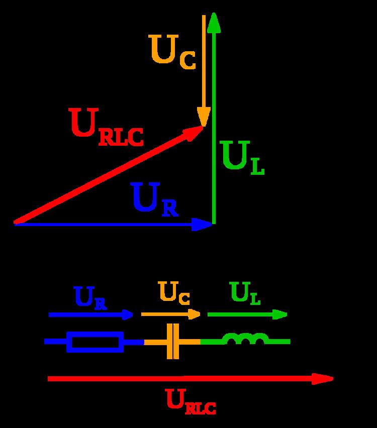This means that for many sources, destructive interference happens when the first and last wave differ by 360 degrees, a full wavelength λ . This is why in single slit diffraction, the minima occurs when light from the far edge travels a full wavelength further than the light from the near edge.

Phasor diagrams

Electrical engineers, electronics engineers, electronic engineering technicians and aircraft engineers all use phasor diagrams to visualize complex constants and variables (phasors). Like vectors, arrows drawn on graph paper or computer displays represent phasors. Cartesian and polar representations each have advantages, with the Cartesian coordinates showing the real and imaginary parts of the phasor and the polar coordinates showing its magnitude and phase.

Circuit laws

With phasors, the techniques for solving DC circuits can be applied to solve AC circuits. A list of the basic laws is given below.

Ohm's law for resistors: a resistor has no time delays and therefore doesn't change the phase of a signal therefore V=IR remains valid.

Ohm's law for resistors, inductors, and capacitors: V = IZ where Z is the complex impedance.

In an AC circuit we have real power (P) which is a representation of the average power into the circuit and reactive power (Q) which indicates power flowing back and forward. We can also define the complex power S = P + jQ and the apparent power which is the magnitude of S. The power law for an AC circuit expressed in phasors is then S = VI^* (where I^* is the complex conjugate of I, and I and V are the RMS values of the voltage and current).

Kirchhoff's circuit laws work with phasors in complex form

Given this we can apply the techniques of analysis of resistive circuits with phasors to analyze single frequency AC circuits containing resistors, capacitors, and inductors. Multiple frequency linear AC circuits and AC circuits with different waveforms can be analyzed to find voltages and currents by transforming all waveforms to sine wave components with magnitude and phase then analyzing each frequency separately, as allowed by the superposition theorem.

Power engineering

In analysis of three phase AC power systems, usually a set of phasors is defined as the three complex cube roots of unity, graphically represented as unit magnitudes at angles of 0, 120 and 240 degrees. By treating polyphase AC circuit quantities as phasors, balanced circuits can be simplified and unbalanced circuits can be treated as an algebraic combination of symmetrical circuits. This approach greatly simplifies the work required in electrical calculations of voltage drop, power flow, and short-circuit currents. In the context of power systems analysis, the phase angle is often given in degrees, and the magnitude in rms value rather than the peak amplitude of the sinusoid.

The technique of synchrophasors uses digital instruments to measure the phasors representing transmission system voltages at widespread points in a transmission network. Differences among the phasors indicate power flow and system stability.

References

Phasor Wikipedia

(Text) CC BY-SA

Contents