
 | ||
In statistics, Deming regression, named after W. Edwards Deming, is an errors-in-variables model which tries to find the line of best fit for a two-dimensional dataset. It differs from the simple linear regression in that it accounts for errors in observations on both the x- and the y- axis. It is a special case of total least squares, which allows for any number of predictors and a more complicated error structure.
Contents
Deming regression is equivalent to the maximum likelihood estimation of an errors-in-variables model in which the errors for the two variables are assumed to be independent and normally distributed, and the ratio of their variances, denoted δ, is known. In practice, this ratio might be estimated from related data-sources; however the regression procedure takes no account for possible errors in estimating this ratio.
The Deming regression is only slightly more difficult to compute compared to the simple linear regression. Most statistical software packages used in clinical chemistry offer Deming regression.
The model was originally introduced by Adcock (1878) who considered the case δ = 1, and then more generally by Kummell (1879) with arbitrary δ. However their ideas remained largely unnoticed for more than 50 years, until they were revived by Koopmans (1937) and later propagated even more by Deming (1943). The latter book became so popular in clinical chemistry and related fields that the method was even dubbed Deming regression in those fields.
Specification
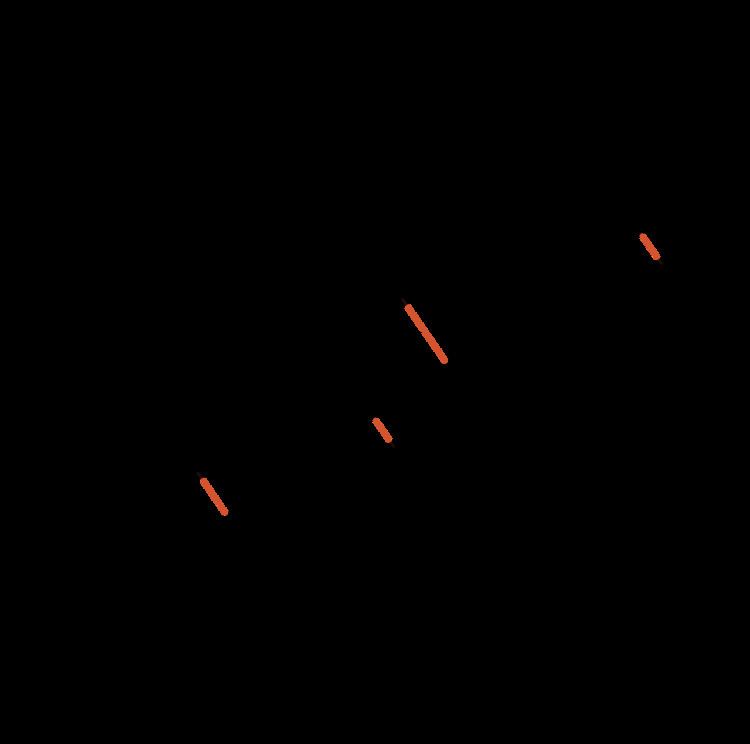
Assume that the available data (yi, xi) are measured observations of the "true" values (yi*, xi*), which lie on the regression line:
where errors ε and η are independent and the ratio of their variances is assumed to be known:
In practice, the variances of the
We seek to find the line of "best fit"
such that the weighted sum of squared residuals of the model is minimized:
Solution
The solution can be expressed in terms of the second-degree sample moments. That is, we first calculate the following quantities (all sums go from i = 1 to n):
Finally, the least-squares estimates of model's parameters will be
Orthogonal regression
For the case of equal error variances, i.e., when
A trigonometric representation of the orthogonal regression line was given by Coolidge in 1913.
Application
In the case of three non-collinear points in the plane, the triangle with these points as its vertices has a unique Steiner inellipse that is tangent to the triangle's sides at their midpoints. The major axis of this ellipse falls on the orthogonal regression line for the three vertices.