DNA read errors

Overview

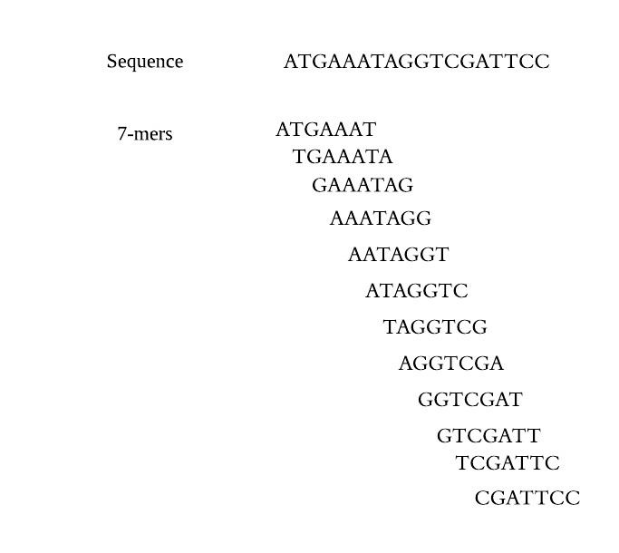
From the way a de Bruijn graph is formed, we can see that there is a possibility of 4^k different nodes to make arrangements of a genome. The number of nodes used to create the graph can be reduced in number by considering only the k-mers found within the DNA strand of interest. Given sequence 1, we can determine the nodes of size 7, or 7-mers, that will be in the graph. These 7-mers then create the graph shown in figure 1.

The graph shown in figure 1 is a very simple version of what a graph could look like... This graph is formed by taking the last 6 elements of the 7-mer and linking it to the node whose first 6 elements are the same. Figure 1 is the most simplistic a de Bruijn graph can be, since each node has exactly one path into it and one path out. Most of the time, you will most likely see a graph where there is more than one edge directed to a node and/or more than one edge leaving a node. This happens due to the way nodes are connected. The nodes are connected by edges pointing to nodes if, and only if, the last k-1 elements of the k-mer you are looking at matches the first k-1 elements of any node. This allows for a multiple-edged de Bruijn graph to form. These more complicated graphs happen due to either read errors or variations in DNA strands. Both causes make it difficult to determine the correct structure of the DNA, and what is causing the differences. Since most DNA strands will likely include read errors and variations, scientists hope to use an assembly process that can merge nodes of the graph when they are unambiguously connected after the graph has been cleaned of vertices and edges created by the errors.

Tips and Bubbles

When a graph is formed from sequenced data, the read errors form tips and bubbles. A tip is where an error occurred during the sequencing process and has caused the graph to end prematurely and includes both correct and incorrect k-mers. A bubble is also formed when an error occurs during the sequence reading process; however, wherever the error happens, there is a path for the k-mer reads to reconnect with the main graph and continue as though nothing had ever happened. When there are tips and bubbles present in a de Bruijn graph formed from the data, they may be removed only if an error is what caused the tip or bubble to appear. When scientists are using a reference genome, they can quickly and easily tell where tips are located by comparing the graph of the reference genome and the graph of the sequence. If there is not a reference genome, these tips are eliminated by tracing the branches backward until a point of ambiguity is found. These tips are then removed only if the branch containing the tip is shorter than a set threshold length. The process of removing bubbles is slightly more complicated. The first thing that needs done is to identify the beginning of the bubble. From there, each path from the beginning of the bubble is followed until the point of reconnection. The point of reconnection can be different for each path. Since there can be paths of various lengths from the beginning node, the path which has a lower coverage is removed.

Example

Given a sequence of any length, the first step that needs done is to enter the sequence into a sequencing program, have it sequenced, and return base pair (bp) reads of a certain length. Since there is not a sequencing program that is completely accurate, there will always be some reads which contain errors. The most common sequencing method is the shotgun method, which is the method most probably used on sequence 2. Once a method is decided on, you have to specify the length of the bp reads you would like it to return. In the case of sequence 2, it returned 7-bp reads with all errors made during the process noted in red.

Once the reads are obtained, they are hashed into k-mers. The k-mers then are recorded in a table with how many times each k-mer appeared in the reads. For this example, each read was hashed into 4-mers and if there was an error it was recorded in red. All of the 4-mers were then recorded, with their frequency in the following table.

Each individual cell of the table will then form a node, allowing a de Bruijn graph to be formed from the given k-mers. In figure 2, linear stretches are identified and then another graph, figure 3, is formed where the linear stretches have become a single node, of a different k-mer size, allowing for a more concise graph. In this simplified graph, it is easy to identify various tips and bubbles, as shown in figure 4. These bubbles and tips can then be removed, since we can identify that they were formed from errors in the bp reads, giving us a graph structure that should accurately and completely reflect the original sequence. If you follow the de Bruijn graph shown in figure 5, you will see that the sequence formed does indeed match the DNA sequence given in sequence 2.

Comparing Two DNA Strands

When comparing two strands of DNA, colored de Bruijn graphs are frequently used to identify errors. These errors, often polymorphisms, cause bubbles, similar to the ones mentioned above, to form. Currently there are four main algorithms used to generalize the data and locate bubbles. The four algorithms extend de Bruijn graphs by allowing the nodes and edges in the graph to be colored by the samples from which they were observed

Bubble Calling

The simplest use of a colored de Bruijn graph is known as the bubble calling algorithm. This algorithm looks, and locates, bubbles on the genome that differ from the original. These bubbles must be “clean”, or simply a divergence from the reference genome, but cannot be caused by deletions of DNA bases. This algorithm can have high false positive rates since there is a difficulty of separating repeat- and variant-induced bubbles; however, there is often a reference genome to help improve reliability. The reference genome also helps in the detection of variants and is essential to detect variant sites. Recently, scientists have discovered a way to use the bubble calling algorithm with copy number variation detection to allow for an opportunity of unbiased detection of these variations in the future

Path Divergence

When looking at complex variants, there is a very low chance that they will make a clean contig. Since this is the case most often, the path divergence algorithm is useful, especially when considering where deletions occur and the variant is so complex it is constrained to the reference allele. When there is a bubble formed, the path divergence algorithm is used the most frequently and allows detected bubbles to get deleted in a very systematic procedure. The algorithm first locates each point of divergence. Then from each point of divergence, the strands that form the bubble are traced to find where the two paths join after n nodes. If the two paths join, then the path with a lower coverage is removed and stored in a file.

Multiple Sample Analysis

Using multiple samples substantially improves the power and false discovery rate of detecting variants. In the simplest cases, the samples are combined into a group of a single color and the data is analyzed as described previously. However, by maintaining separate colors for each sample set, additional information on how the bubbles were formed, whether by error or by repeats, presents itself. In 1997, the Department of Technology Development at Genzyme Genetics in Framingham, Massachusetts developed a new approach that provided a breakthrough in dealing with bubbles using the multiplex allele-specific diagnostic assay (MASDA). This program combines forward dot-blot, complex simultaneous probe hybridization and direct mutation detection to help solve the dual problem of multiple sample analysis.

Genotyping

The colored de Bruijn graphs can be used to genotype any DNA sample at a known loci, even when the coverage is less than sufficient for variant assembly. The first step to this process is to construct a graph of the reference allele, known variants and data from the sample. The algorithm then calculates the likelihood of each genotype and accounts for the structure of the graph, both of the local and genome-wide sequence. This then generalizes to multiple allelic types and helps genotype complex and compound variants. This algorithm is used frequently, as there are no bubbles formed to deal with. This also directly helps find the more complicated issues in genes more direct than any of the three algorithms previously mentioned.