Chinese remainder theorem

History

The earliest known statement of the theorem, as a problem with specific numbers, appears in the 3rd-century book Sunzi Suanjing by the Chinese mathematician Sunzi:

Sunzi's work contains neither a proof nor a full algorithm. What amounts to an algorithm for solving this problem was described by Aryabhata (6th century). Special cases of the Chinese remainder theorem were also known to Brahmagupta (7th century), and appear in Fibonacci's Liber Abaci (1202). The result was later generalized with a complete solution called Dayanshu (大衍術) in Qin Jiushao's 1247 Mathematical Treatise in Nine Sections (數書九章, Shushu Jiuzhang).

The notion of congruences was first introduced and used by Gauss in his Disquisitiones Arithmeticae of 1801. Gauss illustrates the Chinese remainder theorem on a problem involving calendars, namely, "to find the years that have a certain period number with respect to the solar and lunar cycle and the Roman indiction." Gauss introduces a procedure for solving the problem that had already been used by Euler but was in fact an ancient method that had appeared several times.

Theorem statement

Let n₁, ..., n_k be integers greater than 1, which are often called moduli or divisors. Let us denote by N the product of the n_i.

The Chinese remainder theorem asserts that if the n_i are pairwise coprime, and if a₁, ..., a_k are integers such that 0 ≤ a_i < n_i for every i, then there is one and only one integer x, such that 0 ≤ x < N and the remainder of the Euclidean division of x by n_i is a_i for every i.

This may be restated as follows in term of congruences: If the n_i are pairwise coprime, and if a₁, ..., a_k are any integers, then there exists an integer x such that

x ≡ a 1 ( mod n 1 ) ⋮ x ≡ a k ( mod n k ) ,

and any two such x are congruent modulo N.

In abstract algebra, the theorem is often restated as: if the n_i are pairwise coprime, the map

x mod ⁡ N ↦ ( x mod ⁡ n 1 , … , x mod ⁡ n k )

defines a ring isomorphism

Z / N Z ≅ Z / n 1 Z × ⋯ × Z / n k Z

between the ring of integers modulo N and the direct product of the rings of integers modulo the n_i. This means that for doing a sequence of arithmetic operations in Z / N Z , one may do the same computation independently in each Z / n i Z and then get the result by applying the isomorphism (from the right to the left). This may be much faster than the direct computation if N and the number of operations are large. This is widely used, under the name multi-modular computation, for linear algebra over the integers or the rational numbers.

The theorem can also be restated in the language of combinatorics as the fact that the infinite arithmetic progressions of integers form a Helly family.

Proof

The existence and the uniqueness of the solution may be proved independently. However the first proof of existence, given below, uses the uniqueness.

Uniqueness

Suppose that x and y are both solutions to all the congruences. As x and y give the same remainder, when divided by n_i, their difference x − y is a multiple of each n_i. As the n_i are pairwise coprime, their product N divides also x − y, and thus x and y are congruent modulo N. If x and y are supposed to be non negative and less than N (as in the first statement of the theorem), then their difference may be a multiple of N only if x = y.

Existence (first proof)

The map

x ↦ ( x mod ⁡ n 1 , … , x mod ⁡ n k )

maps congruence classes modulo N to sequences of congruence classes modulo n_i. The proof of uniqueness shows that this map is injective. As the domain and the codomain of this map have the same number of elements, the map is also surjective, which proves the existence of the solution.

This proof is very simple, but does not provide any direct way for computing a solution. Moreover, it cannot be generalized to other situations where the following proof can.

Existence (constructive proof)

Existence may be established by an explicit construction of x. This construction may be split in two steps, firstly by solving the problem in the case of two moduli, and the second one by extending this solution to the general case by induction on the number of moduli.

Case of two moduli

We want to solve the system

x ≡ a 1 ( mod n 1 ) x ≡ a 2 ( mod n 2 ) ,

where n 1 and n 2 are coprime.

Bézout's identity asserts the existence of two integers m 1 and m 2 such that

m 1 n 1 + m 2 n 2 = 1.

The integers m 1 and m 2 may be computed by Extended Euclidean algorithm.

A solution is given by

x = a 1 m 2 n 2 + a 2 m 1 n 1 .

In fact

x = a 1 m 2 n 2 + a 2 m 1 n 1 = a 1 m 2 n 2 + a 2 m 1 n 1 + ( a 1 m 1 n 1 − a 1 m 1 n 1 ) = a 1 ( m 1 n 1 + m 2 n 2 ) − a 1 m 1 n 1 + a 2 m 1 n 1 = a 1 + n 1 m 1 ( a 2 − a 1 ) .

This shows that x ≡ a 1 ( mod n 1 ) . The second congruence is proved similarly, by exchanging the indices.

General case

Let us consider a sequence of congruence equations

x ≡ a 1 ( mod n 1 ) ⋮ x ≡ a k ( mod n k ) ,

where the n i are pairwise coprime. The two first equations have a solution a 1 , 2 provided by the method of the previous section. The set of the solutions of these two first equations is the set of all solutions of the equation

x ≡ a 1 , 2 ( mod n 1 n 2 ) .

As the other n i are coprime with n 1 n 2 , this reduces solving the initial problem of k equations to a similar problem with k − 1 equations. Iterating the process, one gets eventually the solutions of the initial problem

Existence (direct construction)

For constructing a solution, it is not necessary to make an induction on the number of moduli. However, such a direct construction involves more computation with large numbers, which makes it less efficient and less used. Nevertheless, Lagrange interpolation is a special case of this construction, applied to polynomials instead of integers.

Let N i = N / n i be the product of all moduli but one. As the n i are pairwise coprime, N i and n i are coprime. Thus Bézout's identity applies, and there exist integers M i and m i such that

M i N i + m i n i = 1.

A solution of the system of congruences is

x = ∑ i = 1 k a i M i N i .

In fact, as N i is a multiple of n j for i ≠ j , we have

x ≡ a i M i N i ≡ a i ( M i N i + m i n i ) − a i m i n i ≡ a i ( mod n i ) ,

for every i .

Computation

Let us consider a system of congruences

x ≡ a 1 ( mod n 1 ) ⋮ x ≡ a k ( mod n k ) ,

where the n i are pairwise coprime, and let N = n 1 n 2 ⋯ n k . In this section several methods are described for computing the unique solution for x , such that 0 ≤ x < N , and these methods are applied on the example

x ≡ 0 ( mod 3 ) x ≡ 3 ( mod 4 ) x ≡ 4 ( mod 5 ) .

Systematic search

It is easy to check whether a value of x is a solution: it suffices to compute the remainder of the Euclidean division of x by each n_i. Thus, to find the solution, it suffices to check successively the integers from 0 to N until finding the solution.

Although very simple this method is very inefficient: for the simple example considered here, 40 integers (including 0) have to be checked for finding the solution 39. This is an exponential time algorithm, as the size of the input is, up to a constant factor, the number of digits of N, and the average number of operations is of the order of N.

Therefore, this method is rarely used, for hand-written computation as well on computers.

Search by sieving

The search of the solution may be made dramatically faster by sieving. For this method, we suppose, without loss of generality, that 0 ≤ a i < n i (if it were not the case, it would suffice to replace each a i by the remainder of its division by n i ). This implies that the solution belongs to the arithmetic progression

a 1 , a 1 + n 1 , a 1 + 2 n 1 , …

By testing the values of these numbers modulo n 2 , one eventually finds a solution x 2 of the two first congruences. Then the solution belongs to the arithmetic progression

x 2 , x 2 + n 1 n 2 , x 2 + 2 n 1 n 2 , …

Testing the values of these numbers modulo n 3 , , and continuing until every modulus has been tested gives eventually the solution.

This method is faster if the moduli have been ordered by decreasing value, that is if n 1 > n 2 > ⋯ > n k . For the example, this gives the following computation. We consider first the numbers that are congruent to 4 modulo 5 (the largest modulus), which are 4, 9 = 4 + 5, 14 = 9 + 5, ... For each of them, compute the remainder by 4 (the second largest modulus) until getting a number congruent to 3 modulo 4. Then one can proceed by adding 20 = 5×4 at each step, and computing only the remainders by 3. This gives

4 mod 4 → 0. Continue 4 + 5 = 9 mod 4 →1. Continue 9 + 5 = 14 mod 4 → 2. Continue 14 + 5 = 19 mod 4 → 3. OK, continue by considering remainders modulo 3 and adding 5×4 = 20 each time 19 mod 3 → 1. Continue 19 + 20 = 39 mod 3 → 0. OK, this is the result.

This method works well for hand-written computation with a product of moduli that is not too big. However it is much slower than other methods, for very large products of moduli. Although dramatically faster than the systematic search, this method has also an exponential time complexity, and is therefore not used on computers.

Using the existence construction

The constructive existence proof shows that, in the case of two moduli, the solution may be obtained by the computation of the Bézout coefficients of the moduli, followed by a few multiplications, additions and reductions modulo n 1 n 2 (for getting a result in the interval ( 0 , n 1 n 2 − 1 ) ). As the Bézout's coefficients may be computed with the extended Euclidean algorithm, the whole computation, at most, has a quadratic time complexity of O ( ( s 1 + s 2 ) 2 ) , where s i denotes the number of digits of n i .

For more than two moduli, the method for two moduli allows the replacement of any two congruences by a single congruence modulo the product of the moduli. Iterating this process provides eventually the solution with a complexity, which is quadratic in the number of digits of the product of all moduli. This quadratic time complexity does not depend on the order in which the moduli are regrouped. One may regroup the two first moduli, then regrouping the resulting modulus with the next one, and so on. This is the strategy which is the easiest to implement, but it needs more computation involving large numbers.

Another strategy consists in partitioning the moduli in pairs whose product have comparable sizes (as much as possible), applying parallely the method of two moduli to each pair, and iterating with a number of moduli approximatively divided by two. This method allows an easy parallelization of the algorithm. Also, if fast algorithms (that is algorithms working in quasilinear time) are used for the basic operations, this method provides an algorithm for the whole computation that works in quasilinear time.

On the current example (which has only three moduli), both strategies are identical, and works as follows.

Bézout's identity for 3 and 4 is

1 × 4 + ( − 1 ) × 3 = 1.

Putting this in the formula given for proving the existence gives

0 × 4 + ( − 3 ) × 3 = − 9

for a solution of the two first congruences, the other solutions being obtained by adding to −9 any multiple of 3×4 = 12. One may continue with any of these solutions, but the solution 3 = −9 +12 is smaller (in absolute value) and thus leads probably to an easier computation

Bézout identity for 5 and 3×4 = 12 is

5 × 5 + ( − 2 ) × 12 = 1.

Applying the same formula again, we get a solution of the problem:

25 × 3 − 24 × 4 = − 21.

The other solutions are obtained by adding any multiple of 3×4×5 = 60, and the smallest positive solution is −21 + 60 = 39.

As a linear Diophantine system

The system of congruences solved by the Chinese remainder theorem may be rewritten as a system of simultaneous linear Diophantine equations

x = a 1 + x 1 n 1 ⋮ x = a k + x k n k ,

where the unknown integers are x and the x i . Therefore, every general method for solving such systems may be used for finding the solution of Chinese remainder theorem, such as the reduction of the matrix of the system to Smith normal form or Hermite normal form. However, as usual when using a general algorithm for a more specific problem, this approach is less efficient than the method of the preceding section, based on a direct use of Bézout's identity.

Over principal ideal domains

In § Theorem statement, the Chinese remainder theorem has been stated in three different ways: in terms of remainders, of congruences and of a ring isomorphism. The statement in terms of remainders does not apply, in general, to principal ideal domains, as remainders are not defined in such rings. However, the two other versions make sense over a principal ideal domain R: it suffices to replace "integer" by "element of the domain" and Z by R. These two versions of the theorem are true in this context, because the proofs (except for the first existence proof), are based on Euclid's lemma and Bézout's identity, which are true over every principal domain.

However, in general, the theorem is only an existence theorem, and does not provide any way for computing the solution, unless one has an algorithm for computing the coefficients of Bézout's identity.

Over univariate polynomial rings and Euclidean domains

The statement in terms of remainders given in § Theorem statement cannot be generalized to any principal ideal domain, but its generalization to Euclidean domains is straightforward. The univariate polynomials over a field is the typical example of a Euclidean domain, which is not the integers. therefore, we state the theorem for the case of a ring of univariate domain R = K [ X ] over a field K . For getting the theorem for a general Euclidean domain, it suffices to replace the degree by the Euclidean function of the Euclidean domain.

The Chinese remainder theorem for polynomials is thus: Let P i ( X ) (the moduli) be, for i=1, ..., k, pairwise coprime polynomials in R = K [ X ] . Let d i = deg ⁡ P i be the degree of P i ( X ) , and D be the sum of the d i . If A i ( X ) , … , A k ( X ) are polynomials such that A i ( X ) = 0 or deg ⁡ A i < d i for every i, then, there is one and only one polynomial P ( X ) , such that deg ⁡ P < D and the remainder of the Euclidean division of P ( X ) by P i ( X ) is A i ( X ) for every i.

The construction of the solution may be done as in § Existence (constructive proof) or § Existence (direct proof). However, the latter construction may be simplified by using, as follows, partial fraction decomposition instead of extended Euclidean algorithm.

Thus, we want to find a polynomial P ( X ) , which satisfies the congruences

P ( X ) ≡ A i ( X ) ( mod P i ( X ) ) ,

for i = 1 , … , k .

Let us consider the polynomials

Q ( X ) = ∏ i = 1 k P i ( X ) Q i ( X ) = Q ( X ) P i ( X ) .

The partial fraction decomposition of 1 / Q ( X ) gives k polynomials S i ( X ) with degrees deg ⁡ S i ( X ) < d i , such that

1 Q ( X ) = ∑ i = 1 k S i ( X ) P i ( X ) ,

and thus

1 = ∑ i = 1 k S i ( X ) Q i ( X ) .

Then a solution of the simultaneous congruence system is given by the polynomial

∑ i = 1 k A i ( X ) S i ( X ) Q i ( X ) .

In fact, we have

∑ i = 1 k A i ( X ) S i ( X ) Q i ( X ) = A i ( X ) + ∑ j = 1 k ( A j ( X ) − A i ( X ) ) S j ( X ) Q j ( X ) ≡ A i ( X ) ( mod P i ( X ) ) ,

for 1 ≤ i ≤ k .

This solution may have a degree larger that D = ∑ i = 1 k d i . The unique solution of degree less than D may be deduced by considering the remainder B i ( X ) of the Euclidean division of A i ( X ) S i ( X ) by P i ( X ) . This solution is

P ( X ) = ∑ i = 1 k B i ( X ) Q i ( X ) .

Lagrange interpolation

A special case of Chinese remainder theorem for polynomials is Lagrange interpolation. For this, let us consider k monic polynomials of degree one:

P i ( X ) = X − x i .

They are pairwise coprime if the x i are all different. The remainder of the division by P i ( X ) of a polynomial P ( X ) is P ( x i ) .

Now, let A 1 , … , A k be constants (polynomials of degree 0) in K . Both Lagrange interpolation and Chinese remainder theorem assert the existence of a unique polynomial P ( X ) , of degree less than k such that

P ( x i ) = A i ,

for every i.

Lagrange interpolation formula is exactly the result, in this case, of the above construction of the solution. More precisely, let

Q ( X ) = ∏ i = 1 k ( X − x i ) Q i ( X ) = Q ( X ) X − x i .

The partial fraction decomposition of 1 / Q ( X ) is

1 Q ( X ) = ∑ i = 1 k 1 Q i ( x i ) ( X − X i ) .

In fact, reducing the right-hand side to a common denominator one gets ∑ i = 1 k 1 Q i ( x i ) ( X − X i ) = ∑ i = 1 k Q i ( X ) / Q i ( x i ) Q ( X ) , and the numerator is equal to one, as being a polynomial of degree less than k, which takes the value one for k different values of X .

Using the above general formula, we get the Lagrange interpolation formula

P ( X ) = ∑ i = 1 k A i Q i ( X ) Q i ( x i ) .

Hermite interpolation

Hermite interpolation is an application of Chinese remainder theorem for univariate polynomials, which may involve moduli of arbitrary degrees (Lagrange interpolation involves only moduli of degree one).

The problem consists of finding a polynomial of the least possible degree, such that the polynomial and its first derivatives take given values at some fixed points.

More precisely, let x 1 , … , x k be k elements of the ground field K , and, for i = 1 , … , k , let a i , 0 , a i , 1 , … , a i , r i − 1 be the values of the first r i derivatives of the sought polynomial at x i (including the 0th derivative, which is the value of the polynomial itself). The problem is to find a polynomial P ( X ) such that its jth derivative takes the value a i , j at x i , for i = 1 , … , k and j = 0 , … , r j .

Let us consider the polynomial

P i ( X ) = ∑ j = 0 r i − 1 a i , j j ! ( X − x i ) j .

This is the Taylor polynomial of order r i − 1 at x i , of the unknown polynomial P ( X ) . Therefore, we must have

P ( X ) ≡ P i ( X ) ( mod ( X − x i ) r i ) .

Conversely, any polynomial P ( X ) that satisfies these k congruences, in particular verifies, for any i = 1 , … , k

P ( X ) = P i ( X ) + o ( X − x i ) r i − 1

therefore P i ( X ) is its Taylor polynomial of order r i − 1 at x i , that is, P ( X ) solves the initial Hermite interpolation problem. The Chinese remainder theorem asserts that there exists exactly one polynomial of degree less than the sum of the r i , which satisfies these k congruences.

There are several ways for computing the solution P ( X ) . One may use the method described at the beginning of § Over univariate polynomial rings and Euclidean domains. One may also use the constructions given in § Existence (constructive proof) or § Existence (direct proof).

Generalization to arbitrary rings

The Chinese remainder theorem can be generalized to any ring, by using coprime ideals (also called comaximal ideals). Two ideals I and J are coprime if there are elements i ∈ I and j ∈ J such that i + j = 1. This relation plays the role of Bézout's identity in the proofs related to this generalization, which, otherwise are very similar. The generalization may be stated as follows.

Let I₁, ..., I_k be two-sided ideals of a ring R that are pairwise coprime, and I be their intersection. Then we have the isomorphism

R / I → R / I 1 × ⋯ × R / I k x mod ⁡ I ↦ ( x mod ⁡ I 1 , ⋯ , x mod ⁡ I k ) ,

between the quotient ring R / I and the direct product of the R / I i , where " x mod ⁡ I " denotes the image of the element x in the quotient ring defined by the ideal I . Moreover, if R is commutative, then the ideal intersection I is equal to the product of the ideals I i :

I = I 1 ∩ I 2 ∩ … ∩ I k = I 1 I 2 ⋯ I k

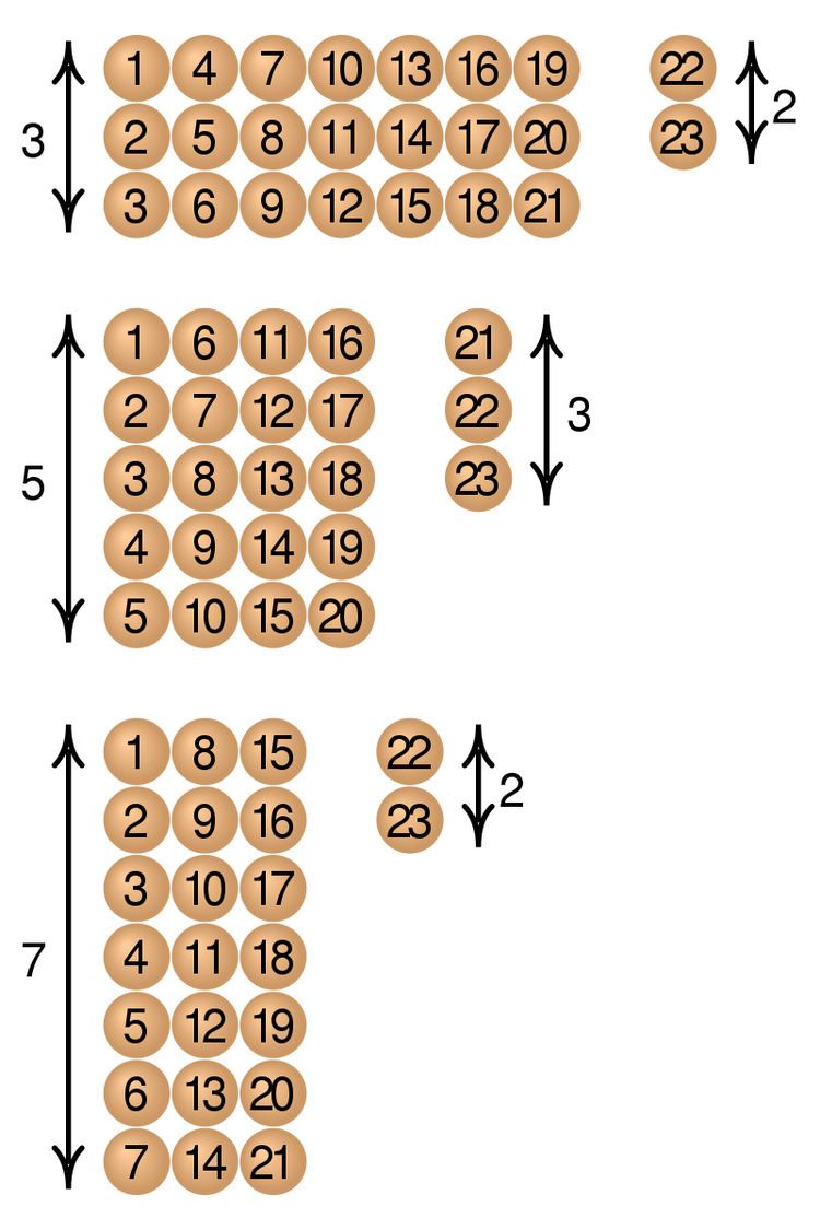
Sequence numbering

The Chinese remainder theorem has been used to construct a Gödel numbering for sequences, which is involved in the proof of Gödel's incompleteness theorems.

Fast Fourier transform

The prime-factor FFT algorithm (also called Good-Thomas algorithm) uses the Chinese remainder theorem for reducing the computation of a fast Fourier transform of size n 1 n 2 to the computation of two fast Fourier transforms of smaller sizes n 1 and n 2 (providing that n 1 and n 2 are coprime).

Encryption

Most implementations of RSA use the Chinese remainder theorem during signing of HTTPS certificates and during decryption.

The Chinese remainder theorem can also be used in secret sharing, which consists of distributing a set of shares among a group of people who, all together (but no one alone), can recover a certain secret from the given set of shares. Each of the shares is represented in a congruence, and the solution of the system of congruences using the Chinese remainder theorem is the secret to be recovered. Secret sharing using the Chinese remainder theorem uses, along with the Chinese remainder theorem, special sequences of integers that guarantee the impossibility of recovering the secret from a set of shares with less than a certain cardinality.

Range ambiguity resolution

The range ambiguity resolution techniques used with medium pulse repetition frequency radar can be seen as a special case of the Chinese remainder theorem.

Dedekind's theorem

Dedekind's Theorem on the Linear Independence of Characters. Let M be a monoid and k an integral domain, viewed as a monoid by considering the multiplication on k. Then any finite family ( f_i )_i∈I of distinct monoid homomorphisms  f_i : M → k is linearly independent. In other words, every family (α_i)_i∈I of elements α_i ∈ k satisfying

∑ i ∈ I α i f i = 0

must be equal to the family (0)_i∈I.

Proof. First assume that k is a field, otherwise, replace the integral domain k by its quotient field, and nothing will change. We can linearly extend the monoid homomorphisms  f_i : M → k to k-algebra homomorphisms F_i : k[M] → k, where k[M] is the monoid ring of M over k. Then, by linearity, the condition

∑ i ∈ I α i f i = 0 ,

yields

∑ i ∈ I α i F i = 0.

Next, for i, j ∈ I; i ≠ j the two k-linear maps F_i : k[M] → k and F_j : k[M] → k are not proportional to each other. Otherwise  f_i  and  f_j  would also be proportional, and thus equal since as monoid homomorphisms they satisfy:  f_i (1) = 1 =  f_j (1), which contradicts the assumption that they are distinct.

Therefore, the kernels Ker F_i and Ker F_j are distinct. Since k[M]/Ker F_i ≅ F_i(k[M]) = k is a field, Ker F_i is a maximal ideal of k[M] for every i ∈ I. Because they are distinct and maximal the ideals Ker F_i and Ker F_j are coprime whenever i ≠ j. The Chinese Remainder Theorem (for general rings) yields an isomorphism:

ϕ : k [ M ] / K → ∏ i ∈ I k [ M ] / K e r F i ϕ ( x + K ) = ( x + K e r F i ) i ∈ I

where

K = ∏ i ∈ I K e r F i = ⋂ i ∈ I K e r F i .

Consequently, the map

Φ : k [ M ] → ∏ i ∈ I k [ M ] / K e r F i Φ ( x ) = ( x + K e r F i ) i ∈ I

is surjective. Under the isomorphisms k[M]/Ker F_i → F_i(k[M]) = k, the map Φ corresponds to:

ψ : k [ M ] → ∏ i ∈ I k ψ ( x ) = [ F i ( x ) ] i ∈ I

Now,

∑ i ∈ I α i F i = 0

yields

∑ i ∈ I α i u i = 0

for every vector (u_i)_i∈I in the image of the map ψ. Since ψ is surjective, this means that

∑ i ∈ I α i u i = 0

for every vector

( u i ) i ∈ I ∈ ∏ i ∈ I k .

Consequently, (α_i)_i∈I = (0)_i∈I. QED.