I am a computer expert who loves a challenge. When I am not managing servers and fixing flaws, I write about it and other interesting things on various blogs.
Cavity optomechanics
Updated on
Edit
Like
Comment
Share
Sign in
Cavity optomechanics nergis mavalvala
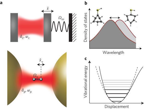
Cavity optomechanics is a branch of physics which focuses on the interaction between light and mechanical objects on low-energy scales. It is a cross field of optics, quantum optics, solid-state physics and materials science. The motivation for research on cavity optomechanics comes from fundamental effects of quantum theory and gravity, as well as technological applications.
The name of the field relates to the main effect of interest, which is the enhancement of radiation pressure interaction between light (photons) and matter using optical resonators (cavities). It first became relevant in the context of gravitational wave detection, since optomechanical effects have to be taken into account in interferometric gravitational wave detectors. Furthermore, one may envision optomechanical structures to allow the realization of Schrödinger's cat. Macroscopic objects consisting of billions of atoms share collective degrees of freedom which may behave quantum mechanically, e.g. a sphere of micrometer diameter being in a spatial superposition between two different places. Such a quantum state of motion would allow to experimentally investigate decoherence, which describes the process of objects transitioning between states which are described by quantum mechanics to states which are described by Newtonian mechanics. Optomechanical structures pave a new way for testing the predictions of quantum mechanics and decoherence models and thereby might allow to answer some of the most fundamental questions in modern physics.
There is a broad range of experimental optomechanical systems which are almost equivalent in their description, but completely different in size, mass and frequency, ranging from attograms and gigahertz to kilograms and hertz. Cavity optomechanics was featured as the most recent milestone of photon history in nature photonics along well established concepts and technology like Quantum information, Bell inequalities and the laser.
Quantum cavity optomechanics part i by nikolai kiesel
Physical processes
The most elementary light-matter interaction is the light beam scattering off an arbitrary object (atom, molecule, nanobeam etc.). There is always elastic light scattering, with the outgoing light frequency identical to the incoming frequency ω′=ω. Inelastic scattering, in contrast, will be accompanied by excitation or de-excitation of the material object (e.g. internal atomic transitions may be excited). However, independent of the internal electronic details of the atoms or molecules, it is always possible to have Raman scattering due to the object's mechanical vibrations:
ω′=ω±ωm,
where ωm is the vibrational frequency. The vibrations gain or lose energy, respectively, for these Stokes/anti-Stokes processes, while optical sidebands are created around the incoming light frequency, i.e.
ω′=ω∓ωm.
If both of these processes (Stokes and anti-Stokes scattering) occur at an equal rate, the vibrations will merely heat up the object. However, one may use an optical cavity to suppress e.g. the Stokes process. This reveals the principle of the basic optomechanical setup: A laser-driven optical cavity is coupled to the mechanical vibrations of some object. This is a very generic setting. The purpose of the cavity is to select optical frequencies (e.g. to suppress the Stokes process), to resonantly enhance the light intensity and to enhance the sensitivity to the mechanical vibrations. This setup displays features of a true two-way interaction between light and mechanics. This is in contrast to optical tweezers, optical lattices, or vibrational spectroscopy, where the light field controls the mechanics (or vice versa) but the loop is not closed.
Another but equivalent way to interpret the principle of optomechanical cavities is by using the concept of radiation pressure. According to the quantum theory of light, every photon with wave number k carries a momentum p=ℏk with Planck's constant ℏ. This means that a photon, which is reflected off a mirror surface, transfers a momentum Δp=2ℏk onto the mirror due to the conservation of momentum. This effect is extremely small and can not be observed on most every-day objects, however it becomes more significant when the mass of the mirror is very small and/or the number of photons is very large (i.e. high intensity of the light). Since the momentum of photons is extremely small and not enough to change the position of a suspended mirror significantly, one needs to enhance the interaction. One possible way to do this is by using optical cavities. If a photon is enclosed between two mirrors, one being the oscillator and the other a heavy fixed one, it will bounce off the mirrors many times and transfer its momentum every time it hits the mirrors. The number of times a photon can transfer its momentum is directly related to the finesse of the cavity, which can be improved with highly reflective mirror surfaces. To understand why this radiation pressure of the photons does not simply shift the suspended mirror further and further away, one has to take into account the effect on the cavity light field: If the mirror is displaced, the cavity becomes longer (or shorter) which changes the cavity resonance frequency. Thus the detuning between the changed cavity and the unchanged laser driving frequency is modified. This detuning determines the light amplitude inside the cavity - at smaller detuning more light actually enters the cavity, because it is closer to the cavity resonance frequency. Since the light amplitude, i.e. the number of photons inside the cavity, causes the radiation pressure force and thus the displacement of the mirror we have closed the loop: The radiation pressure force effectively depends on the mirror position. Another advantage of optical cavities is that the modulation of the cavity length through an oscillating mirror can directly be seen in the spectrum of the cavity.
Some first effects of the light on the mechanical resonator can be captured by converting the radiation pressure force into a potential,
ddxVrad(x)=−F(x),
and adding it to the intrinsic harmonic oscillator potential of the mechanical oscillator. This combined potential reveals the possibility of static multi-stability in the system, i.e. the potential can feature several stable minima. In addition, the slope of the radiation pressure force F(x) can be understood as a modification of the mechanical spring constant,
D=D0−dFdx.
This effect is known as optical spring effect (light-induced spring constant).
However, this picture is not complete, as it neglects retardation effects due to the finite cavity photon decay rate κ. The force follows the motion of the mirror only with some time delay. This leads to effects such as friction. For example, let us assume the equilibrium position sit somewhere on the rising slope of the resonance. In thermal equilibrium, there will be oscillations around this position, which do not follow the shape of the resonance because of retardation. The consequence of this delayed radiation force during one cycle of oscillation turns out to be that work is carried out, in this particular case it is negative,∮Fdx<0, i.e. the radiation force extracts mechanical energy (there is extra, light-induced damping). This can be used to cool down the mechanical motion and is referred to as optical or optomechanical cooling. It is important for reaching the quantum regime of the mechanical oscillator where thermal noise effects on the device become negligible. Similarly, if the equilibrium position sits on the falling slope of the cavity resonance, the work is positive and the mechanical motion is amplified. In this case the extra, light-induced damping is negative and leads to amplification of the mechanical motion (heating). Radiation-induced damping of this kind has first been observed in pioneering experiments by Braginsky and coworkers in 1970.
Another explanation for the basic optomechanical effects of cooling and amplification can be given in a quantized picture. By detuning the incoming light from the cavity resonance to the red sideband, the photons can only enter the cavity if they take phonons with energy ℏωm from the mechanics. This effectively cools the device until a balance with heating mechanisms from the environment and laser noise is reached. In the same fashion it is also possible to heat structures (amplify the mechanical motion) by detuning the driving laser to the blue side. In this case the laser photons scatter into a cavity photon and create an additional phonon in the mechanical oscillator.
In general, one can divide the basic behaviour of the optomechanical system into different regimes, depending on the detuning between the laser frequency and the cavity resonance frequency,
Δ=ωL−ωcav:
Red-detuned regimeΔ<0 (most prominent effects on the red sideband Δ=−ωm): In this regime state exchange between two resonant oscillators can occur (i.e. a beam-splitter in quantum optics language). This can be used for state transfer between phonons and photons (which requires the so-called ”strong coupling regime”) or the above-mentioned optical cooling.
Blue-detuned regimeΔ>0 (most prominent effects on the blue sideband Δ=+ωm): This regime describes "two-mode squeezing". It can be used to achieve entanglement, squeezing, and mechanical "lasing" (amplification of the mechanical motion to self-sustained optomechanical oscillations / limit cycle oscillations), if the growth of the mechanical energy overwhelms the intrinsic losses (mainly mechanical friction).
On-resonance regimeΔ=0: In this regime the cavity is simply operated as an interferometer, so it can be used to read out the mechanical motion.
Also the optical spring effect depends on the detuning. It can be observed for large detuning Δ≫ωm,κ and its strength varies with detuning and the laser drive.
Hamiltonian
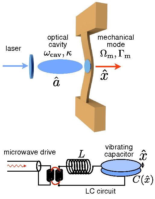
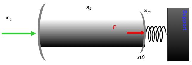
The standard optomechanical setup is a Fabry–Pérot cavity, where one mirror is movable and thus provides an additional mechanical degree of freedom. Mathematically this system can be described by a single optical cavity mode coupled to a single mechanical mode. The coupling originates from the radiation pressure of the light field, that eventually moves the mirror a little bit, thus changing the cavity length and resonance frequency. The optical mode is driven by an external laser. This system can be described by the following effective Hamiltonian
Htot=ℏωcav(x)a†a+ℏωmb†b+iℏE(aeiωLt−a†e−iωLt)
where a and b are the bosonic annihilation operators of the given cavity mode and the mechanical resonator respectively, satisfying the commutation relations
[a,a†]=[b,b†]=1.
ωcav is the frequency of the optical mode, now dependant on the position x of the mechanical resonator, whereas ωm is the mechanical mode frequency. The last term describes the driving, with ωL the driving laser frequency and E the amplitude, given by
E=PκℏωL
with P the input power coupled to the optical mode under consideration and κ its linewidth. Of course, the system is coupled to the environment so the full treatment of the system should also include optical and mechanical dissipation (denoted by κ and Γ respectively) and the corresponding noise entering the system.
The standard optomechanical Hamiltonian is obtained by getting rid of the explicit time dependence of the laser driving term and separating the optomechanical interaction from the free optical oscillator. This is achieved by switching into a reference frame rotating at the laser frequency ωL (in which case the optical mode annihilation operator undergoes the transformation a→ae−iωLt) and applying a Taylor expansion on ωcav. Quadratic and higher order coupling terms are usually neglected, such that the standard Hamiltonian becomes
Htot=−ℏΔa†a+ℏωmb†b−ℏg0a†axxzpf+iℏE(a−a†)
with Δ=ωL−ωcav the laser detuning and the position operator x=xzpf(b+b†). The first two terms are the free optical and mechanical Hamiltonian respectively. The third term contains the optomechanical interaction, with g0=dωcavdx|x=0xzpf the single-photon optomechanical coupling strength (sometimes also called the bare optomechanical coupling). It determines by how much the cavity resonance frequency is shifted if the mechanical oscillator is displaced by the zero point uncertainty xzpf=ℏ/2meffωm. Here, meff is the effective mass of the mechanical oscillator. Sometimes, it is more convenient to use G=g0/xzpf instead, which determines the frequency change per displacement of the mirror, also called frequency pull parameter.
E.g., for a Fabry–Pérot cavity of length L with a moving end-mirror the optomechanical coupling strength can directly be determined from the geometry to be g0=ωcav(0)xzpf/L.
This mathematical description using Htot is based on the assumption that only one optical and mechanical mode interact. Each optical cavity supports in principle an infinite number of modes and mechanical oscillators have more than a single oscillation/vibration mode. The validity of this approach relies on the possibility to tune the laser in such a way, that it populates a single optical mode only (that implies that the spacing between the cavity modes needs to be sufficiently large). Furthermore, scattering of photons to other modes is supposed to be negligible, which holds if the mechanical (motional) sidebands of the driven mode do not overlap with other cavity modes, i.e. if the mechanical mode frequency is smaller than the typical separation of the optical modes.
Linearization
Usually, the single-photon optomechanical coupling strength g0 is a small frequency, much smaller than the cavity decay rate κ, but the effective optomechanical coupling can be enhanced by increasing the drive power. Namely, with a strong enough drive, the dynamics of the system can be considered as quantum fluctuations around a classical steady state, i.e. a=α+δa, where α is the mean light field amplitude and δa denotes the fluctuations. Expanding the photon number a†a, we can omit the term α2 as it leads to a constant radiation pressure force which simply shifts the resonator's equilibrium position. Also neglecting the second order term δa†δa, we obtain the linearized optomechanical Hamiltonian,
Hlin=−ℏΔδa†δa+ℏωmb†b−ℏg(δa+δa†)(b+b†)
where g=g0α. This Hamiltonian is quadratic in operators, but it is called linearized, because it leads to linear equations of motion. It is a valid description of many experiments, where g0 is typically very small and needs to be enhanced by the driving laser. Again, for a realistic description dissipation should be added to both the optical and the mechanical oscillator. The driving term from the standard Hamiltonian is not part of the linearized Hamiltonian, since it is the source of the classical light amplitude α around which the linearization was executed.
With a particular choice of detuning, different phenomena can be observed (see also the section about physical processes). The clearest distinction can be made between the following three cases:
Δ≈−ωm: In this case a rotating wave approximation of the linearized Hamiltonian, where one omits all non-resonant terms, reduces the coupling Hamiltonian to a beamsplitter operator, Hint=ℏg0(δa†b+δab†). This approximation works best on resonance, i.e. if the detuning becomes exactly equal to the negative mechanical frequency. Negative detuning (red detuning of the laser from the cavity resonance) by an amount equal to the mechanical mode frequency favors the anti-Stokes sideband, leading to a net cooling of the resonator. Laser photons absorb energy from the mechanical oscillator by annihilating phonons in order to become resonant with the cavity.
Δ≈ωm: In this case a rotating wave approximation of the linearized Hamiltonian leads to other resonant terms. The coupling Hamiltonian takes the form Hint=ℏg0(δab+δa†b†), which is proportional to the two-mode squeezing operator. Therefore, two-mode squeezing and entanglement between the mechanical and optical modes can be observed with this parameter choice. Positive detuning (blue detuning of the laser from the cavity resonance) can also lead to instability. In the mechanical sideband picture, this corresponds to enhancing the Stokes sideband, i.e. the laser photons shed energy, increasing the number of phonons and becoming resonant with the cavity in the process.
Δ=0: In this case of driving on-resonance, one has to consider all terms in Hint=ℏg0(δa+δa†)(b+b†). The optical mode experiences a shift proportional to the mechanical displacement, which translates into a phase shift of the light transmitted through (or reflected off) the cavity. Thus, the cavity serves as an interferometer augmented by the factor of the optical finesse and can be used to measure very small displacements. (In fact, this setup has recently enabled LIGO to detect gravitational waves.)
Equations of motion
From the linearized Hamiltonian one can, adding dissipation and noise terms to the Heisenberg equations of motion, derive the so-called linearized quantum Langevin equations, which govern the dynamics of the optomechanical system.
δa˙=(iΔ−κ/2)δa+ig(b+b†)−κain
b˙=−(iωm+Γ/2)b+ig(δa+δa†)−Γbin
Here ain and bin are the input noise operators (either quantum or thermal noise) and −κδa and −Γδp are the corresponding dissipative terms. Note that for optical photons, thermal noise can be neglected due to the high frequencies, such that the optical input noise can be described by quantum noise only (this does not hold for microwave implementations of the optomechanical system). For the mechanical oscillator thermal noise has to be taken into account and is the reason why many experiments are placed in additional cooling environments to lower the ambient temperature.
Rewritten in frequency space (i.e. a Fourier transform is applied), these first order differential equations become easily solvable.
Two main effects of the light on the mechanical oscillator can then be expressed in the following way:
δωm=g2(Δ−ωmκ2/4+(Δ−ωm)2+Δ+ωmκ2/4+(Δ+ωm)2)
Γeff=Γ+g2(κκ2/4+(Δ+ωm)2−κκ2/4+(Δ−ωm)2)
The former is termed the optical-spring effect and may lead to significant frequency shifts in the case of low-frequency oscillators, such as pendulum mirrors. In the case of higher resonance frequencies, ωm≳1 MHz, it does not significantly alter the frequency. For a harmonic oscillator, the relation between a frequency shift and a change in the spring constant originates from Hooke's law.
The latter equation shows optical damping, i.e. the intrinsic mechanical damping Γ becomes stronger (or weaker) due to the optomechanical interaction. From the formula one can see that for negative detuning and large coupling, the mechanical damping can be greatly increased, which corresponds to cooling of the mechanical oscillator. In the case of positive detuning the optomechanical interaction leads to a negative contribution to the effective damping. This can lead to instability, when the effective damping drops below zero, Γeff<0, which means that it turns into an overall amplification rather than a damping of the mechanical oscillator.
Important parameter regimes
The most basic regimes in which the optomechanical system can be operated are defined by the laser detuning Δ and described above. The resulting phenomenas are basically either cooling or heating of the mechanical oscillator. However, additional parameters determine what effects can actually be observed.
The good/bad cavity regime (also called the resolved/unresolved sideband regime) relates the mechanical frequency to the optical linewidth: The good cavity regime (resolved sideband limit) is of experimental relevance since it is a necessary requirement to achieve ground-state cooling of the mechanical oscillator, i.e. cooling to an average mechanical occupation number below 1. The name "resolved sideband regime" refers to the possibility to distinguish the motional sidebands from the cavity resonance, which is the case if the linewidth of the cavity, κ is smaller than the distance from the cavity resonance to the sideband, which is ωm. This requirement leads to a condition for the so-called sideband parameter: ωm/κ≫1. If ωm/κ≪1 the system resides in the bad cavity regime (unresolved sideband limit). Here, the motional sideband lies within the peak of the cavity resonance. Actually, deep in the unresolved sideband regime, many motional sidebands can be included in the broad cavity linewidth, thus e.g. allowing a single photon to create more than one phonon, which leads to larger amplification of the mechanical oscillator.
Another distinction can be made depending on the optomechanical coupling strength. If the (enhanced) optomechanical coupling becomes larger than the cavity linewidth, g≥κ one enters the so-called strong-coupling regime. There the optical and mechanical modes hybridize and normal-mode splitting occurs. This regime has to be distinguished from the (experimentally much more challenging) single-photon strong-coupling regime, where the bare optomechanical coupling becomes of the order of the cavity linewidth, g0≥κ. Only in this regime, effects of the full non-linear interaction described by ℏg0a†a(b+b†) become observable. For example, it is a precondition to create non-Gaussian states with the optomechanical system. Typical experiments currently operate in the linearized regime (small g0≪κ) thus investigating only effects of the linearized Hamiltonian.
Setup
The strength of the optomechanical Hamiltonian is the large range of experimental implementations to which it can be applied. This results in wide parameter ranges for the optomechanical parameters. For example, the size of optomechanical systems can be micrometers but also of the order of kilometers as it is the case for LIGO (although LIGO is dedicated to the detection of gravitational waves and not the investigation of optomechanics specifically).
Examples of real optomechanical implementations are:
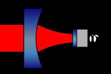
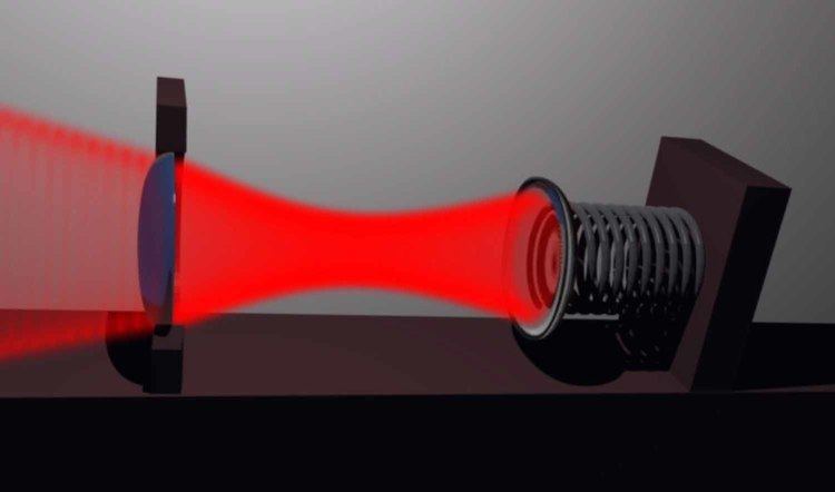
Cavities with a moving mirror: This is the archetype of an optomechanical system. The light is reflected from the mirrors, transferring momentum onto the movable one, which in turn changes the cavity resonance frequency.
Membrane-in-the-middle system: A membrane is brought into a cavity consisting of fixed massive mirrors. The membrane takes now the role of the mechanical oscillator. Depending on the positioning of the membrane inside the cavity this system behaves like the typical optomechanical system.
Microtoroids that support an optical whispering gallery mode can be either coupled to a mechanical mode of the toroid or evanescently to a nanobeam that is brought in proximity.
Optomechanical crystal structures: Patterned dielectrics can confine both optical and mechanical (acoustic) modes in the same area, which leads to an optomechanical interaction.
Electromechanical implementations of an optomechanical system use superconducting LC circuits with a mechanically compliant capacitance using e.g. a micromechanical membrane. Here the role of the optical light is replaced by microwaves. Physics is exactly the same as in optical cavities but the range of parameters is different.
One purpose of studying so many different designs of the same system is the different parameter regimes that are accessible by different setups and their different potential to be converted into tools of commercial use.
Measurement
The optomechanical system can be measured using e.g. a homodyne detection scheme. Either the light of the driving laser is measured, or a two-mode scheme is followed where a strong laser is used to drive the optomechanical system into the state of interest and a second laser is used for the read-out of the state of the system. This second “probe” laser is typically weak, i.e. its optomechanical interaction can be neglected as compared to the effects caused by the strong “pump” laser.
The optical output field can also be measured with single photon detectors e.g. to achieve photon counting statistics.
Relation to fundamental research
One of the questions which are still subject to current debate is the exact mechanism of decoherence. As Schrödinger pointed out, we would never see something like a cat in a quantum state. There needs to be something like a collapse of the quantum wave functions, which brings it from a quantum state to a pure classical state. Now one can ask where the boundary lies between objects with quantum properties and classical objects. Taking spatial superpositions as an example, there might be a size limit to objects which can be brought into superpositions, there might be a limit to the spatial separation of the centers of mass of a superposition or even a limit to the superposition of gravitational fields and its impact on small test masses. Those predictions could be checked with large mechanical structures which can be manipulated at the quantum level.
Some easier to check predictions of quantum mechanics are the prediction of negative Wigner functions for certain quantum states, measurement precision beyond the standard quantum limit using squeezed states of light or the asymmetry of the sidebands in the spectrum of a cavity near the quantum ground state.
Applications
Years before cavity optomechanics gained the status of an independent field of research, many of its techniques were already used in Gravitational wave detectors where it is necessary to measure displacements of mirrors on the order of the Planck scale. Even if these detectors do not address the measurement of quantum effects, they encounter related issues (photon shot noise) and use similar tricks (squeezed coherent states) to enhance the precision. Further applications include the development of quantum memory for quantum computers, high precision sensors (e.g. acceleration sensors) and quantum transducers e.g. between the optical and the microwave domain (taking advantage of the fact that the mechanical oscillator can easily couple to both frequency regimes).
Related fields and expansions
In addition to the above explained standard cavity optomechanics there exist variations of this simplest model:
pulsed optomechanics: The continuous laser driving is replaced by a pulsed driving scheme. This has, for example, advantages when creating entanglement and allows backaction-evading measurements.
quadratic coupling: Going beyond the linear coupling term g0=dωcav(x)dx|x=0xzpf a system with quadratic optomechanical coupling can be investigated. The interaction Hamiltonian would then feature a term ℏgquada†a(b+b†)2 with gsq=12d2ωcav(x)dx2|x=0xzpf2. In membrane-in-the-middle setups it is possible to achieve quadratic coupling in the absence of linear coupling by positioning the membrane at an extremum of the standing wave inside the cavity. One possible application is to carry out a quantum nondemolition measurement of the phonon number.
reversed dissipation regime: In the standard optomechanical system the mechanical damping is much smaller than the optical damping. However, one can engineer a system where this hierarchy is reversed, i.e. the optical damping is much smaller than the mechanical damping, κ≪Γ. As long as one resides within in the linearized regime symmetry implies an inversion of the above described effects: E.g. cooling of the mechanical oscillator in the standard optomechanical system is replaced by cooling of the optical oscillator in a system with reversed dissipation hierarchy. This effect was also seen in optical fiber loops in the 1970s.
dissipative coupling: Here the coupling between optics and mechanics arises from a position-dependent optical dissipation rate κ(x) (instead of a position-dependent cavity resonance frequency ωcav). This changes the interaction Hamiltonian and alters many effects of the standard optomechanical system. E.g. this scheme allows to cool the mechanical resonator to its ground state without the requirement of the good cavity regime.
Extensions to the standard optomechanical system include coupling to more and physically different systems:
optomechanical arrays: Coupling several optomechanical systems to each other (e.g. using evanescent coupling of the optical modes) one can study multi-mode phenomena (e.g. synchronization,…). So far many theoretical predictions have been made, but only few experiments exist. The first optomechanical array (with more than two coupled systems) consists of 7 optomechanical systems.
hybrid systems: An optomechanical system can be coupled to a system of different nature (e.g. a cloud of ultracold atoms, a two-level system,…). This can lead to new effects on both the optomechanical and the additional system.
Cavity optomechanics is closely related to trapped ion physics and Bose–Einstein condensates. These systems share very similar Hamiltonians, but they have less particles (about 10 for ion traps and 105-108 for BECs) interacting with the field of light. It is also related to the field of cavity quantum electrodynamics.