Langevin equation - Alchetron, The Free Social Encyclopedia

In statistical physics, a Langevin equation (Paul Langevin, 1908) is a stochastic differential equation describing the time evolution of a subset of the degrees of freedom. These degrees of freedom typically are collective (macroscopic) variables changing only slowly in comparison to the other (microscopic) variables of the system. The fast (microscopic) variables are responsible for the stochastic nature of the Langevin equation.

Brownian motion as a prototype

The original Langevin equation describes Brownian motion, the apparently random movement of a particle in a fluid due to collisions with the molecules of the fluid,

m d 2 x d t 2 = − λ d x d t + η ( t ) .

The degree of freedom of interest here is the position x of the particle, m denotes the particle's mass. The force acting on the particle is written as a sum of a viscous force proportional to the particle's velocity (Stokes' law), and a noise term η ( t ) (the name given in physical contexts to terms in stochastic differential equations which are stochastic processes) representing the effect of the collisions with the molecules of the fluid. The force η ( t ) has a Gaussian probability distribution with correlation function

⟨ η i ( t ) η j ( t ′ ) ⟩ = 2 λ k B T δ i , j δ ( t − t ′ ) ,

where k B is Boltzmann's constant, T is the temperature and η i ( t ) is the i-th component of the vector η ( t ) . The δ-function form of the correlations in time means that the force at a time t is assumed to be completely uncorrelated with it at any other time. This is an approximation; the actual random force has a nonzero correlation time corresponding to the collision time of the molecules. However, the Langevin equation is used to describe the motion of a "macroscopic" particle at a much longer time scale, and in this limit the δ -correlation and the Langevin equation become exact.

Another prototypical feature of the Langevin equation is the occurrence of the damping coefficient λ in the correlation function of the random force, a fact also known as Einstein relation.

Mathematical aspects

A strictly δ -correlated fluctuating force η ( t ) isn't a function in the usual mathematical sense and even the derivative d x / d t isn't defined in this limit. The Langevin equation as it stands requires an interpretation in this case, see Itō calculus.

Generic Langevin equation

There is a formal derivation of a generic Langevin equation from classical mechanics. This generic equation plays a central role in the theory of critical dynamics, and other areas of nonequilibrium statistical mechanics. The equation for Brownian motion above is a special case.

An essential condition of the derivation is a criterion dividing the degrees of freedom into the categories slow and fast. For example, local thermodynamic equilibrium in a liquid is reached within a few collision times. But it takes much longer for densities of conserved quantities like mass and energy to relax to equilibrium. Densities of conserved quantities, and in particular their long wavelength components, thus are slow variable candidates. Technically this division is realized with the Zwanzig projection operator, the essential tool in the derivation. The derivation is not completely rigorous because it relies on (plausible) assumptions akin to assumptions required elsewhere in basic statistical mechanics.

Let A = { A i } denote the slow variables. The generic Langevin equation then reads

d A i d t = k B T ∑ j [ A i , A j ] d H d A j − ∑ j λ i , j ( A ) d H d A j + ∑ j d λ i , j ( A ) d A j + η i ( t ) .

The fluctuating force η i ( t ) obeys a Gaussian probability distribution with correlation function

⟨ η i ( t ) η j ( t ′ ) ⟩ = 2 λ i , j ( A ) δ ( t − t ′ ) .

This implies the Onsager reciprocity relation λ i , j = λ j , i for the damping coefficients λ . The dependence d λ i , j / d A j of λ on A is negligible in most cases. The symbol H = − l n ( p 0 ) denotes the Hamiltonian of the system, where p 0 ( A ) is the equilibrium probability distribution of the variables A . Finally, [ A i , A j ] is the projection of the Poisson bracket of the slow variables A i and A j onto the space of slow variables.

In the Brownian motion case one would have H = p 2 / ( 2 m k B T ) , A = { p } or A = { x , p } and [ x i , p j ] = δ i , j . The equation of motion d x / d t = p / m for x is exact, there is no fluctuating force η x and no damping coefficient λ x , p .

Harmonic oscillator in a fluid

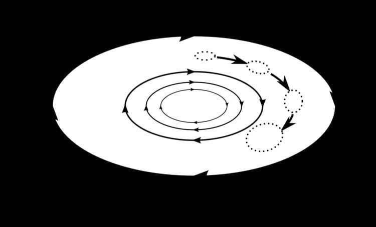
A non-ideal harmonic oscillator is affected by some form of damping, from which it follows via the fluctuation-dissipation theorem that there must be some fluctuations in the system. The diagram at right shows a phase portrait of the time evolution of the momentum, p = m v , vs. position, r of a harmonic oscillator. Deterministic motion would follow along the ellipsoidal trajectories which cannot cross each other without changing energy. The presence of some form of damping, e.g. a molecular fluid environment (represented by diffusion and damping terms), continually adds and removes kinetic energy from the system, causing an initial ensemble of stochastic oscillators (dotted circles) to spread out, eventually reaching thermal equilibrium.

Thermal noise in an electrical resistor

There is a close analogy between the paradigmatic Brownian particle discussed above and Johnson noise, the electric voltage generated by thermal fluctuations in every resistor. The diagram at the right shows an electric circuit consisting of a resistance R and a capacitance C. The slow variable is the voltage U between the ends of the resistor. The Hamiltonian reads H = E / k B T = C U 2 / ( 2 k B T ) , and the Langevin equation becomes

d U d t = − U R C + η ( t ) , ⟨ η ( t ) η ( t ′ ) ⟩ = 2 k B T R C 2 δ ( t − t ′ ) .

This equation may be used to determine the correlation function

⟨ U ( t ) U ( t ′ ) ⟩ = ( k B T / C ) exp ⁡ ( − | t − t ′ | / R C ) ≈ 2 R k B T δ ( t − t ′ ) ,

which becomes a white noise (Johnson noise) when the capacitance C becomes negligibly small.

Critical dynamics

The dynamics of the order parameter φ of a second order phase transition slows down near the critical point and can be described with a Langevin equation. The simplest case is the universality class "model A" with a non-conserved scalar order parameter, realized for instance in axial ferromagnets,

∂ φ ( x , t ) ∂ t = − λ δ H δ φ + η ( x , t ) , H = ∫ d d x { 1 2 φ [ r 0 − ∇ 2 ] φ + u φ 4 } , ⟨ η ( x , t ) η ( x ′ , t ′ ) ⟩ = 2 λ δ ( x − x ′ ) δ ( t − t ′ ) .

Other universality classes (the nomenclature is "model A",..., "model J") contain a diffusing order parameter, order parameters with several components, other critical variables and/or contributions from Poisson brackets.

Recovering Boltzmann statistics

Langevin equations must reproduce the Boltzmann distribution. 1-dimensional overdamped Brownian motion is an instructive example. The overdamped case is realized when the inertia of the particle is negligible in comparison to the damping force. The trajectory x ( t ) of the particle in a potential V ( x ) is described by the Langevin equation

λ d x d t = − ∂ V ( x ) ∂ x + η ( t ) ,

where the noise is characterized by ⟨ η ( t ) η ( t ′ ) ⟩ = 2 k B T λ δ ( t − t ′ ) and λ is the damping constant. We would like to compute the distribution p ( x ) of the particle's position in the course of time. A direct way to determine this distribution is to introduce a test function f , and to look at the average of this function over all realizations (ensemble average)

λ d ⟨ f ( x ( t ) ) ⟩ d t = ⟨ f ′ ( x ( t ) ) λ d x d t ⟩ = ⟨ − f ′ ( x ( t ) ) ∂ V ∂ x + f ′ ( x ( t ) ) η ( t ) ⟩ .

If x ( t ) remains finite then this quantity is null. Moreover, using the Stratonovich interpretation, we are able to get rid of the eta in the second term so that we end up with

⟨ − f ′ ( x ) ∂ V ∂ x + k B T f ″ ( x ) ⟩ = 0 ,

where we make use of the probability density function p ( x ) . This is done by explicitly computing the average,

∫ ( − f ′ ( x ) ∂ V ∂ x p ( x ) + k B T f ″ ( x ) p ( x ) ) d x = ∫ ( − f ′ ( x ) ∂ V ∂ x p ( x ) − k B T f ′ ( x ) p ′ ( x ) ) d x = 0 ,

where the second term was integrated by parts (hence the negative sign). Since this is true for arbitrary functions f , we must have:

∂ V ∂ x p ( x ) + k B T p ′ ( x ) = 0 ,

thus recovering the Boltzmann distribution

p ( x ) ∝ exp ⁡ ( − V ( x ) k B T ) .

Equivalent techniques

A solution of a Langevin equation for a particular realization of the fluctuating force is of no interest by itself, what is of interest are correlation functions of the slow variables after averaging over the fluctuating force. Such correlation functions also may be determined with other (equivalent) techniques.

Fokker Planck equation

A Fokker–Planck equation is a deterministic equation for the time dependent probability density P ( A , t ) of stochastic variables A . The Fokker–Planck equation corresponding to the generic Langevin equation above may be derived with standard techniques (see for instance ref.),

∂ P ( A , t ) ∂ t = ∑ i , j ∂ ∂ A i ( − k B T [ A i , A j ] ∂ H ∂ A j + λ i , j ∂ H ∂ A j + λ i , j ∂ ∂ A j ) P ( A , t ) .

The equilibrium distribution P ( A ) = p 0 ( A ) = c o n s t × exp ⁡ ( − H ) is a stationary solution.

Path integral

A path integral equivalent to a Langevin equation may be obtained from the corresponding Fokker–Planck equation or by transforming the Gaussian probability distribution P ( η ) ( η ) d η of the fluctuating force η to a probability distribution of the slow variables, schematically P ( A ) d A = P ( η ) ( η ( A ) ) det ( d η / d A ) d A . The functional determinant and associated mathematical subtleties drop out if the Langevin equation is discretized in the natural (causal) way, where A ( t + Δ t ) − A ( t ) depends on A ( t ) but not on A ( t + Δ t ) . It turns out to be convenient to introduce auxiliary response variables A ~ . The path integral equivalent to the generic Langevin equation then reads

∫ P ( A , A ~ ) d A d A ~ = N ∫ exp ⁡ ( L ( A , A ~ ) ) d A d A ~ ,

where N is a normalization factor and

L ( A , A ~ ) = ∫ ∑ i , j { A ~ i λ i , j A ~ j − A ~ i { δ i , j d A j d t − k B T [ A i , A j ] d H d A j + λ i , j d H d A j − d λ i , j d A j } } d t .

The path integral formulation doesn't add anything new, but it does allow for the use of tools from quantum field theory; for example perturbation and renormalization group methods (if these make sense).

References

Langevin equation Wikipedia

(Text) CC BY-SA

Contents