Bremsstrahlung

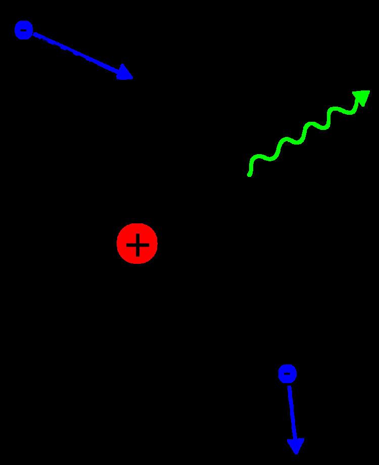
Particle in vacuum

A charged particle accelerating in a vacuum radiates power, as described by the Larmor formula and its relativistic generalizations. Although the term, bremsstrahlung, is usually reserved for charged particles accelerating in matter, not vacuum, the formulas are similar. (In this respect, bremsstrahlung differs from Cherenkov radiation, another kind of braking radiation which occurs only in matter, and not in a vacuum.)

Total radiated power

The most established relativistic formula for total radiated power is given by

P = q 2 γ 4 6 π ε 0 c ( β ˙ 2 + ( β → ⋅ β → ˙ ) 2 1 − β 2 ) ,

where β → = v → / c (the velocity of the particle divided by the speed of light), γ = 1 1 − β 2 is the Lorentz factor, β → ˙ signifies a time derivative of β → , and q is the charge of the particle. This is commonly written in the mathematically equivalent form using ( β → ⋅ β → ˙ ) 2 = β → 2 ⋅ β → ˙ 2 − ( β → × β → ˙ ) 2 :

P = q 2 γ 6 6 π ε 0 c ( β ˙ 2 − ( β → × β → ˙ ) 2 ) .

In the case where velocity is parallel to acceleration (for example, linear motion), the formula simplifies to

P a ∥ v = q 2 a 2 γ 6 6 π ε 0 c 3 ,

where a ≡ v ˙ = β ˙ c is the acceleration. For the case of acceleration perpendicular to the velocity ( β → ⋅ β → ˙ = 0 ) (a case that arises in circular particle accelerators known as synchrotrons), the total power radiated reduces to

P a ⊥ v = q 2 a 2 γ 4 6 π ε 0 c 3 .

radiated in the two limiting cases is proportional to γ 4 ( a ⊥ v ) or γ 6 ( a ∥ v ) . Since E = γ m c 2 , we see that the total radiated power goes as m − 4 or m − 6 , which accounts for why electrons lose energy to bremsstrahlung radiation much more rapidly than heavier charged particles (e.g., muons, protons, alpha particles). This is the reason a TeV energy electron-positron collider (such as the proposed International Linear Collider) cannot use a circular tunnel (requiring constant acceleration), while a proton-proton collider (such as the Large Hadron Collider) can utilize a circular tunnel. The electrons lose energy due to bremsstrahlung at a rate ( m p / m e ) 4 ≈ 10 13 times higher than protons do.

Angular distribution

The most general formula for radiated power as a function of angle is:

d P d Ω = q 2 16 π 2 ε 0 c | n ^ × ( ( n ^ − β → ) × β → ˙ ) | 2 ( 1 − n ^ ⋅ β → ) 5

where n ^ is a unit vector pointing from the particle towards the observer, and d Ω is an infinitesimal bit of solid angle.

In the case where velocity is parallel to acceleration (for example, linear motion), this simplifies to

d P a ∥ v d Ω = q 2 a 2 16 π 2 ε 0 c 3 sin 2 ⁡ θ ( 1 − β cos ⁡ θ ) 5

where θ is the angle between a → and the direction of observation.

Thermal bremsstrahlung

NOTE: this article currently gives formulas that apply in the Rayleigh-Jeans limit ℏ ω ≪ k B T e , and does not use a quantized (Planck) treatment of radiation. Thus a usual factor like exp ⁡ ( − ℏ ω / k B T e ) does not appear. The appearance of ℏ ω / k B T e in y below is due to the quantum-mechanical treatment of collisions.

In a plasma, the free electrons continually collide with the ions, producing bremsstrahlung. A complete analysis requires accounting for both binary Coulomb collisions as well as collective (dielectric) behavior. A detailed treatment is given by Bekefi, while a simplified one is given by Ichimaru. In this section we follow Bekefi's dielectric treatment, with collisions included approximately via the cutoff wavenumber, k m .

Consider a uniform plasma, with thermal electrons distributed according to the Maxwell–Boltzmann distribution with the temperature T e . Following Bekefi, the power spectral density (power per angular frequency interval per volume, integrated over the whole 4 π sr of solid angle, and in both polarizations) of the bremsstrahlung radiated, is calculated to be

d P B r d ω = 8 2 3 π [ e 2 4 π ϵ 0 ] 3 1 ( m e c 2 ) 3 / 2 [ 1 − ω p 2 ω 2 ] 1 / 2 Z i 2 n i n e ( k B T e ) 1 / 2 E 1 ( y ) ,

where ω p ≡ ( n e e 2 / ϵ 0 m e ) 1 / 2 is the electron plasma frequency, ω is the photon frequency, n e , n i is the number density of electrons and ions, and other symbols are physical constants. The second bracketed factor is the index of refraction of a light wave in a plasma, and shows that emission is greatly suppressed for ω < ω p (this is the cutoff condition for a light wave in a plasma; in this case the light wave is evanescent). This formula thus only applies for ω > ω p . This formula should be summed over ion species in a multi-species plasma.

The special function E 1 is defined in the exponential integral article, and the unitless quantity y is

y = 1 2 ω 2 m e k m 2 k B T e

k m is a maximum or cutoff wavenumber, arising due to binary collisions, and can vary with ion species. Roughly, k m = 1 / λ B when k B T e > Z i 2 E h (typical in plasmas that are not too cold), where E h ≈ 27.2 eV is the Hartree energy, and λ B = ℏ / ( m e k B T e ) 1 / 2 is the electron thermal de Broglie wavelength. Otherwise, k m ∝ 1 / l c where l c is the classical Coulomb distance of closest approach.

For the usual case k m = 1 / λ B , we find

y = 1 2 [ ℏ ω k B T e ] 2 .

The formula for d P B r / d ω is approximate, in that it neglects enhanced emission occurring for ω slightly above ω p .

In the limit y ≪ 1 , we can approximate E1 as E 1 ( y ) ≈ − ln ⁡ [ y e γ ] + O ( y ) where γ ≈ 0.577 is the Euler–Mascheroni constant. The leading, logarithmic term is frequently used, and resembles the Coulomb logarithm that occurs in other collisional plasma calculations. For y > e − γ the log term is negative, and the approximation is clearly inadequate. Bekefi gives corrected expressions for the logarithmic term that match detailed binary-collision calculations.

The total emission power density, integrated over all frequencies, is

P B r = ∫ ω p ∞ d ω d P B r d ω = 16 3 [ e 2 4 π ϵ 0 ] 3 1 m e 2 c 3 Z i 2 n i n e k m G ( y p ) G ( y p ) = 1 2 π ∫ y p ∞ d y y − 1 2 [ 1 − y p y ] 1 2 E 1 ( y ) y p = y ( ω = ω p ) G ( y p = 0 ) = 1 and decreases with y p ; it is always positive. For k m = 1 / λ B , we find P B r = 16 3 ( e 2 4 π ϵ 0 ) 3 ( m e c 2 ) 3 2 ℏ Z i 2 n i n e ( k B T e ) 1 2 G ( y p )

Note the appearance of ℏ due to the quantum nature of λ B . In practical units, a commonly used version of this formula for G = 1 is

P B r [ W / m 3 ] = Z i 2 n i n e [ 7.69 × 10 18 m − 3 ] 2 T e [ eV ] 1 2 .

This formula is 1.59 times the one given above, with the difference due to details of binary collisions. Such ambiguity is often expressed by introducing Gaunt factor g B , e.g. in one finds

ε f f = 1.4 × 10 − 27 T 1 2 n e n i Z 2 g B ,

where everything is expressed in the CGS units.

Relativistic corrections

For very high temperatures there are relativistic corrections to this formula, that is, additional terms of the order of k B T e / m e c 2 . [3]

Bremsstrahlung cooling

If the plasma is optically thin, the bremsstrahlung radiation leaves the plasma, carrying part of the internal plasma energy. This effect is known as the bremsstrahlung cooling. It is a type of radiative cooling. The energy carried away by bremsstrahlung is called bremsstrahlung losses and represents a type of radiative losses. One generally uses the term bremsstrahlung losses in the context when the plasma cooling is undesired, as e.g. in fusion plasmas.

Polarizational bremsstrahlung

Polarizational bremsstrahlung (sometimes referred to as "atomic bremsstrahlung") is the radiation emitted by the target's atomic electrons as the target atom is polarized by the Coulomb field of the incident charged particle. Polarizational bremsstrahlung contributions to the total bremsstrahlung spectrum have been observed in experiments involving relatively massive incident particles, resonance processes, and free atoms. However, there is still some debate as to whether or not there are significant polarizational bremsstrahlung contributions in experiments involving fast electrons incident on solid targets.

It is worth noting that the term "polarizational" is not meant to imply that the emitted bremsstrahlung is polarized. Also, the angular distribution of polarizational bremsstrahlung is theoretically quite different than ordinary bremsstrahlung.

Quantum mechanical description

The complete quantum mechanical description was first performed by Bethe and Heitler. They assumed plane waves for electrons which scatter at the nucleus of an atom, and derived a cross section which relates the complete geometry of that process to the frequency of the emitted photon. The quadruply differential cross section which shows a quantum mechanical symmetry to pair production, is:

d 4 σ = Z 2 α fine 3 ℏ 2 ( 2 π ) 2 | p f | | p i | d ω ω d Ω i d Ω f d Φ | q | 4 × [ p f 2 sin 2 ⁡ Θ f ( E f − c | p f | cos ⁡ Θ f ) 2 ( 4 E i 2 − c 2 q 2 ) + p i 2 sin 2 ⁡ Θ i ( E i − c | p i | cos ⁡ Θ i ) 2 ( 4 E f 2 − c 2 q 2 ) + 2 ℏ 2 ω 2 p i 2 sin 2 ⁡ Θ i + p f 2 sin 2 ⁡ Θ f ( E f − c | p f | cos ⁡ Θ f ) ( E i − c | p i | cos ⁡ Θ i ) − 2 | p i | | p f | sin ⁡ Θ i sin ⁡ Θ f cos ⁡ Φ ( E f − c | p f | cos ⁡ Θ f ) ( E i − c | p i | c 1 cos ⁡ Θ i ) ( 2 E i 2 + 2 E f 2 − c 2 q 2 ) ] .

There Z is the atomic number, α fine ≈ 1 / 137 the fine structure constant, ℏ the reduced Planck's constant and c the speed of light. The kinetic energy E kin , i / f of the electron in the initial and final state is connected to its total energy E i , f or its momenta p i , f via

E i , f = E kin , i / f + m e c 2 = m e 2 c 4 + p i , f 2 c 2 ,

where m e is the mass of an electron. Conservation of energy gives

E f = E i − ℏ ω ,

where ℏ ω is the photon energy. The directions of the emitted photon and the scattered electron are given by

Θ i = ∢ ( p i , k ) , Θ f = ∢ ( p f , k ) , Φ = Angle between the planes  ( p i , k )  and  ( p f , k ) ,

where k is the momentum of the photon.

The differentials are given as

d Ω i = sin ⁡ Θ i   d Θ i , d Ω f = sin ⁡ Θ f   d Θ f .

The absolute value of the virtual photon between the nucleus and electron is

− q 2 = − | p i | 2 − | p f | 2 − ( ℏ c ω ) 2 + 2 | p i | ℏ c ω cos ⁡ Θ i − 2 | p f | ℏ c ω cos ⁡ Θ f + 2 | p i | | p f | ( cos ⁡ Θ f cos ⁡ Θ i + sin ⁡ Θ f sin ⁡ Θ i cos ⁡ Φ ) .

The range of validity is given by the Born approximation

v ≫ Z c 137

where this relation has to be fulfilled for the velocity v of the electron in the initial and final state.

For practical applications (e.g. in Monte Carlo codes) it can be interesting to focus on the relation between the frequency ω of the emitted photon and the angle between this photon and the incident electron. Köhn and Ebert integrated the quadruply differential cross section by Bethe and Heitler over Φ and Θ f and obtained:

d 2 σ ( E i , ω , Θ i ) d ω d Ω i = ∑ j = 1 6 I j

with

I 1 = 2 π A Δ 2 2 + 4 p i 2 p f 2 sin 2 ⁡ Θ i ln ⁡ ( Δ 2 2 + 4 p i 2 p f 2 sin 2 ⁡ Θ i − Δ 2 2 + 4 p i 2 p f 2 sin 2 ⁡ Θ i ( Δ 1 + Δ 2 ) + Δ 1 Δ 2 − Δ 2 2 − 4 p i 2 p f 2 sin 2 ⁡ Θ i − Δ 2 2 + 4 p i 2 p f 2 sin 2 ⁡ Θ i ( Δ 1 − Δ 2 ) + Δ 1 Δ 2 ) × [ 1 + c Δ 2 p f ( E i − c p i cos ⁡ Θ i ) − p i 2 c 2 sin 2 ⁡ Θ i ( E i − c p i cos ⁡ Θ i ) 2 − 2 ℏ 2 ω 2 p f Δ 2 c ( E i − c p i cos ⁡ Θ i ) ( Δ 2 2 + 4 p i 2 p f 2 sin 2 ⁡ Θ i ) ] , I 2 = − 2 π A c p f ( E i − c p i cos ⁡ Θ i ) ln ⁡ ( E f + p f c E f − p f c ) , I 3 = 2 π A ( Δ 2 E f + Δ 1 p f c ) 2 + 4 m 2 c 4 p i 2 p f 2 sin 2 ⁡ Θ i × ln ⁡ [ ( [ E f + p f c ] [ 4 p i 2 p f 2 sin 2 ⁡ Θ i ( E f − p f c ) + ( Δ 1 + Δ 2 ) ( [ Δ 2 E f + Δ 1 p f c ] − [ Δ 2 E f + Δ 1 p f c ] 2 + 4 m 2 c 4 p i 2 p f 2 sin 2 ⁡ Θ i ) ] ) [ ( E f − p f c ) ( 4 p i 2 p f 2 sin 2 ⁡ Θ i [ − E f − p f c ] + ( Δ 1 − Δ 2 ) ( [ Δ 2 E f + Δ 1 p f c ] − ( Δ 2 E f + Δ 1 p f c ) 2 + 4 m 2 c 4 p i 2 p f 2 sin 2 ⁡ Θ i ] ) ] − 1 ] × [ − ( Δ 2 2 + 4 p i 2 p f 2 sin 2 ⁡ Θ i ) ( E f 3 + E f p f 2 c 2 ) + p f c ( 2 [ Δ 1 2 − 4 p i 2 p f 2 sin 2 ⁡ Θ i ] E f p f c + Δ 1 Δ 2 [ 3 E f 2 + p f 2 c 2 ] ) ( Δ 2 E f + Δ 1 p f c ) 2 + 4 m 2 c 4 p i 2 p f 2 sin 2 ⁡ Θ i − c ( Δ 2 E f + Δ 1 p f c ) p f ( E i − c p i cos ⁡ Θ i ) − 4 E i 2 p f 2 ( 2 [ Δ 2 E f + Δ 1 p f c ] 2 − 4 m 2 c 4 p i 2 p f 2 sin 2 ⁡ Θ i ) ( Δ 1 E f + Δ 2 p f c ) ( [ Δ 2 E f + Δ 1 p f c ] 2 + 4 m 2 c 4 p i 2 p f 2 sin 2 ⁡ Θ i ) 2 + 8 p i 2 p f 2 m 2 c 4 sin 2 ⁡ Θ i ( E i 2 + E f 2 ) − 2 ℏ 2 ω 2 p i 2 sin 2 ⁡ Θ i p f c ( Δ 2 E f + Δ 1 p f c ) + 2 ℏ 2 ω 2 p f m 2 c 3 ( Δ 2 E f + Δ 1 p f c ) ( E i − c p i cos ⁡ Θ i ) ( [ Δ 2 E f + Δ 1 p f c ] 2 + 4 m 2 c 4 p i 2 p f 2 sin 2 ⁡ Θ i ) ] , I 4 = − 4 π A p f c ( Δ 2 E f + Δ 1 p f c ) ( Δ 2 E f + Δ 1 p f c ) 2 + 4 m 2 c 4 p i 2 p f 2 sin 2 ⁡ Θ i − 16 π E i 2 p f 2 A ( Δ 2 E f + Δ 1 p f c ) 2 ( [ Δ 2 E f + Δ 1 p f c ] 2 + 4 m 2 c 4 p i 2 p f 2 sin 2 ⁡ Θ i ) 2 , I 5 = 4 π A ( − Δ 2 2 + Δ 1 2 − 4 p i 2 p f 2 sin 2 ⁡ Θ i ) ( [ Δ 2 E f + Δ 1 p f c ] 2 + 4 m 2 c 4 p i 2 p f 2 sin 2 ⁡ Θ i ) × [ ℏ 2 ω 2 p f 2 E i − c p i cos ⁡ Θ i × E f ( 2 Δ 2 2 [ Δ 2 2 − Δ 1 2 ] + 8 p i 2 p f 2 sin 2 ⁡ Θ i [ Δ 2 2 + Δ 1 2 ] ) + p f c ( 2 Δ 1 Δ 2 [ Δ 2 2 − Δ 1 2 ] + 16 Δ 1 Δ 2 p i 2 p f 2 sin 2 ⁡ Θ i ) Δ 2 2 + 4 p i 2 p f 2 sin 2 ⁡ Θ i + 2 ℏ 2 ω 2 p i 2 sin 2 ⁡ Θ i ( 2 Δ 1 Δ 2 p f c + 2 Δ 2 2 E f + 8 p i 2 p f 2 sin 2 ⁡ Θ i E f ) E i − c p i cos ⁡ Θ i + 2 E i 2 p f 2 ( 2 [ Δ 2 2 − Δ 1 2 ] [ Δ 2 E f + Δ 1 p f c ] 2 + 8 p i 2 p f 2 sin 2 ⁡ Θ i [ ( Δ 1 2 + Δ 2 2 ) ( E f 2 + p f 2 c 2 ) + 4 Δ 1 Δ 2 E f p f c ] ) ( Δ 2 E f + Δ 1 p f c ) 2 + 4 m 2 c 4 p i 2 p f 2 sin 2 ⁡ Θ i + 8 p i 2 p f 2 sin 2 ⁡ Θ i ( E i 2 + E f 2 ) ( Δ 2 p f c + Δ 1 E f ) E i − c p i cos ⁡ Θ i ] , I 6 = 16 π E f 2 p i 2 sin 2 ⁡ Θ i A ( E i − c p i cos ⁡ Θ i ) 2 ( − Δ 2 2 + Δ 1 2 − 4 p i 2 p f 2 sin 2 ⁡ Θ i ) ,

and

A = Z 2 α fine 3 ( 2 π ) 2 | p f | | p i | ℏ 2 ω Δ 1 = − p i 2 − p f 2 − ( ℏ c ω ) 2 + 2 ℏ c ω | p i | cos ⁡ Θ i , Δ 2 = − 2 ℏ c ω | p f | + 2 | p i | | p f | cos ⁡ Θ i .

However, a much simpler expression for the same integral can be found in (Eq. 2BN) and in (Eq. 4.1).

An analysis of the doubly differential cross section above shows that electrons whose kinetic energy is larger than the rest energy (511 keV) emit photons in forward direction while electrons with a small energy emit photons isotropically.

Electron-electron bremsstrahlung

One mechanism which is important for small atomic numbers Z , is the scattering of a free electron at the shell electrons of an atom or molecule. Since electron-electron bremsstrahlung is a function of Z and the usual electron-nucleus bremsstrahlung is a function of Z 2 , electron-electron bremsstrahlung is negligible for metals. For air, however, it plays an important role in the production of terrestrial gamma-ray flashes.