Biot–Savart law

Electric currents (along closed curve)

The Biot–Savart law is used for computing the resultant magnetic field B at position r generated by a steady current I (for example due to a wire): a continual flow of charges which is constant in time and the charge neither accumulates nor depletes at any point. The law is a physical example of a line integral, being evaluated over the path C in which the electric currents flow. The equation in SI units is

where d l is a vector whose magnitude is the length of the differential element of the wire in the direction of conventional current, r ′ = r − l , the full displacement vector from the wire element ( l ) to the point at which the field is being computed ( r ), and μ₀ is the magnetic constant. Alternatively:

where r ^ ′ is the unit vector of r ′ . The symbols in boldface denote vector quantities.

The integral is usually around a closed curve, since electric currents can only flow around closed paths. An infinitely long wire (as used in the definition of the SI unit of electric current - the Ampere) is a counter-example.

To apply the equation, the point in space where the magnetic field is to be calculated is arbitrarily chosen ( r ). Holding that point fixed, the line integral over the path of the electric currents is calculated to find the total magnetic field at that point. The application of this law implicitly relies on the superposition principle for magnetic fields, i.e. the fact that the magnetic field is a vector sum of the field created by each infinitesimal section of the wire individually.

There is also a 2D version of the Biot-Savart equation, used when the sources are invariant in one direction. In general, the current need not flow only in a plane normal to the invariant direction and it is given by J . The resulting formula is:

Electric currents (throughout conductor volume)

The formulations given above work well when the current can be approximated as running through an infinitely-narrow wire. If the conductor has some thickness, the proper formulation of the Biot–Savart law (again in SI units) is:

or, alternatively:

where d V is the volume element and J is the current density vector in that volume (in SI in units of A/m²).

The Biot–Savart law is fundamental to magnetostatics, playing a similar role to Coulomb's law in electrostatics. When magnetostatics does not apply, the Biot–Savart law should be replaced by Jefimenko's equations.

Constant uniform current

In the special case of a steady constant current I, the magnetic field B is

i.e. the current can be taken out of the integral.

Point charge at constant velocity

In the case of a point charged particle q moving at a constant velocity v, Maxwell's equations give the following expression for the electric field and magnetic field:

where r ^ ′ is the unit vector pointing from the current (non-retarded) position of the particle to the point at which the field is being measured, and θ is the angle between v and r ′ .

When v² ≪ c², the electric field and magnetic field can be approximated as

These equations are called the "Biot–Savart law for a point charge" due to its closely analogous form to the "standard" Biot–Savart law given previously. These equations were first derived by Oliver Heaviside in 1888.

Magnetic responses applications

The Biot–Savart law can be used in the calculation of magnetic responses even at the atomic or molecular level, e.g. chemical shieldings or magnetic susceptibilities, provided that the current density can be obtained from a quantum mechanical calculation or theory.

Aerodynamics applications

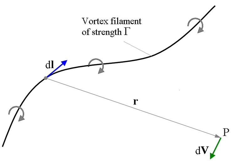
The Biot–Savart law is also used in aerodynamic theory to calculate the velocity induced by vortex lines.

In the aerodynamic application, the roles of vorticity and current are reversed in comparison to the magnetic application.

In Maxwell's 1861 paper 'On Physical Lines of Force', magnetic field strength H was directly equated with pure vorticity (spin), whereas B was a weighted vorticity that was weighted for the density of the vortex sea. Maxwell considered magnetic permeability μ to be a measure of the density of the vortex sea. Hence the relationship,

The electric current equation can be viewed as a convective current of electric charge that involves linear motion. By analogy, the magnetic equation is an inductive current involving spin. There is no linear motion in the inductive current along the direction of the B vector. The magnetic inductive current represents lines of force. In particular, it represents lines of inverse square law force.

In aerodynamics the induced air currents are forming solenoidal rings around a vortex axis that is playing the role that electric current plays in magnetism. This puts the air currents of aerodynamics into the equivalent role of the magnetic induction vector B in electromagnetism.

In electromagnetism the B lines form solenoidal rings around the source electric current, whereas in aerodynamics, the air currents form solenoidal rings around the source vortex axis.

Hence in electromagnetism, the vortex plays the role of 'effect' whereas in aerodynamics, the vortex plays the role of 'cause'. Yet when we look at the B lines in isolation, we see exactly the aerodynamic scenario in so much as that B is the vortex axis and H is the circumferential velocity as in Maxwell's 1861 paper.

In two dimensions, for a vortex line of infinite length, the induced velocity at a point is given by

where Γ is the strength of the vortex and r is the perpendicular distance between the point and the vortex line.

This is a limiting case of the formula for vortex segments of finite length:

where A and B are the (signed) angles between the line and the two ends of the segment.

The Biot–Savart law, Ampère's circuital law, and Gauss's law for magnetism

In a magnetostatic situation, the magnetic field B as calculated from the Biot–Savart law will always satisfy Gauss's law for magnetism and Ampère's law:

In a non-magnetostatic situation, the Biot–Savart law ceases to be true (it is superseded by Jefimenko's equations), while Gauss's law for magnetism and the Maxwell–Ampère law are still true.