Algorithmic cooling

Overview

Quantum computers need qubits (quantum bits) on which they operate. Generally, in order to make the computation more reliable, the qubits must be as pure as possible, minimizing possible fluctuations. Since the purity of a qubit is related to von Neumann entropy and to temperature, making the qubits as pure as possible is equivalent to making them as cold as possible (or having as little entropy as possible). One method of cooling qubits is extracting entropy from them, thus purifying them. This can be done in two general ways: reversibly (namely, using unitary operations) or irreversibly (for example, using a heat bath). Algorithmic cooling is the name of a family of algorithms that are given a set of qubits and purify (cool) a subset of them to a desirable level.

This can also be viewed in a probabilistic manner. Since qubits are two-level systems, they can be regarded as coins, unfair ones in general. Purifying a qubit means (in this context) making the coin as unfair as possible: increasing the difference between the probabilities for tossing different results as much as possible. Moreover, the entropy previously mentioned can be viewed using the prism of information theory, which assigns entropy to any random variable. The purification can therefore be considered as using probabilistic operations (such as classical logical gates and conditional probability) for minimizing the entropy of the coins, making them more unfair.

The case in which the algorithmic method is reversible, such that the total entropy of the system is not changed, was first named "molecular scale heat engine", and is also named "reversible algorithmic cooling". This process cools some qubits while heating the others. It is limited by a variant of Shannon's bound on data compression and it can asymptotically reach quite close to the bound.

A more general method, "irreversible algorithmic cooling", makes use of irreversible transfer of heat outside of the system and into the environment (and therefore may bypass the Shannon bound). Such an environment can be a heat bath, and the family of algorithms which use it is named "heat-bath algorithmic cooling". In this algorithmic process entropy is transferred reversibly to specific qubits (named reset spins) that are coupled with the environment much more strongly than others. After a sequence of reversible steps that let the entropy of these reset qubits increase they become hotter than the environment. Then the strong coupling results in a heat transfer (irreversibly) from these reset spins to the environment. The entire process may be repeated and may be applied recursively to reach low temperatures for some qubits.

Thermodynamics

Algorithmic cooling can be discussed using classical and quantum thermodynamics points of view.

Cooling

The classical interpretation of "cooling" is transferring heat from one object to the other. However, the same process can be viewed as entropy transfer. For example, if two gas containers that are both in thermal equilibrium with two different temperatures are put in contact, entropy will be transferred from the "hotter" object (with higher entropy) to the "colder" one. This approach can be used when discussing the cooling of an object whose temperature is not always intuitively defined, e.g. a single particle. Therefore, the process of cooling spins can be thought of as a process of transferring entropy between spins, or outside of the system.

Heat reservoir

The concept of heat reservoir is discussed extensively in classical thermodynamics (for instance in carnot cycle). For the purposes of algorithmic cooling, it is sufficient to consider heat reservoirs, or "heat baths", as large objects whose temperature remains unchanged even when in contact with other ("normal" sized) objects. Intuitively, this can be pictured as a bath filled with room-temperature water that practically retains its temperature even when a small piece of hot metal is put in it.

Using the entropy form of thinking from the previous subsection, an object which is considered hot (whose entropy is large) can transfer heat (and entropy) to a colder heat bath, thus lowering its own entropy. This process results in cooling.

Unlike entropy transfer between two "regular" objects which preserves the entropy of the system, entropy transfer to a heat bath is normally regarded as non-preserving. This is because the bath is normally not considered as a part of the relevant system, due to its size. Therefore, when transferring entropy to a heat bath, one can essentially lower the entropy of their system, or equivalently, cool it. Continuing this approach, the goal of algorithmic cooling is to reduce as much as possible the entropy of the system of qubits, thus cooling it.

General introduction

Algorithmic cooling applies to quantum systems. Therefore, it is important to be familiar with both the core principles and the relevant notations.

A qubit (or quantum bit) is a unit of information that can be in a superposition of two states, denoted as | 0 ⟩ and | 1 ⟩ . The general superposition can be written as | ψ ⟩ = α | 0 ⟩ + β | 1 ⟩ , where | α | 2 + | β | 2 = 1 and α , β ∈ C . If one measures the state of the qubit in the orthonormal basis composed of | 0 ⟩ and | 1 ⟩ , one gets the result | 0 ⟩ with probability | α | 2 and the result | 1 ⟩ with probability | β | 2 .

The above description is known as a quantum pure state. A general mixed quantum state can be prepared as a probability distribution over pure states, and is represented by a density matrix of the general form ρ = ∑ i p i | ψ i ⟩ ⟨ ψ i | , where each | ψ i ⟩ is a pure state (see ket-bra notations) and each p i is the probability of | ψ i ⟩ in the distribution. The quantum states that play a major role in algorithmic cooling are mixed states in the diagonal form ρ = ( 1 + ϵ 2 0 0 1 − ϵ 2 ) for ϵ ∈ [ − 1 , 1 ] . Essentially, this means that the state is the pure | 0 ⟩ state with probability 1 + ϵ 2 and is pure | 1 ⟩ with probability 1 − ϵ 2 . In the ket-bra notations, the density matrix is 1 + ϵ 2 | 0 ⟩ ⟨ 0 | + 1 − ϵ 2 | 1 ⟩ ⟨ 1 | . For ϵ = ± 1 the state is called pure, and for ϵ = 0 the state is called completely mixed (represented by the normalized identity matrix). The completely mixed state represents a uniform probability distribution over the states | 0 ⟩ and | 1 ⟩ .

Polarization or bias of a state

The state ρ above is called ϵ -polarized, or ϵ -biased, since it deviates by ϵ in the diagonal entries from the completely mixed state.

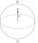
Another approach for the definition of bias or polarization is using Bloch sphere (or generally Bloch ball). Restricted to a diagonal density matrix, a state can be on the straight line connecting the antipodal points representing the states | 0 ⟩ and | 1 ⟩ ("north and south poles" of the sphere). In this approach, the ϵ parameter ( ϵ ∈ [ − 1 , 1 ] ) is exactly the distance (up to a sign) of the state from the center of the ball, which represents the completely mixed state. For ϵ = ± 1 the state is exactly on the poles and for ϵ = 0 the state is exactly in the center. A bias can be negative (for example − 1 2 ), and in this case the state is in the middle between the center and the south pole.

In the Puali-matrices representation form, an ϵ -biased quantum state is ρ = 1 2 ( 1 + ϵ 0 0 1 − ϵ ) = 1 2 ( I + ( 0 , 0 , ϵ ) ⋅ σ → ) = 1 2 ( I + ϵ σ z ) .

Entropy

Since quantum systems are involved, the entropy used here is von Neumann entropy. For a single qubit represented by the (diagonal) density matrix above, its entropy is H ( ϵ ) = − ( 1 + ϵ 2 log ⁡ 1 + ϵ 2 + 1 − ϵ 2 log ⁡ 1 − ϵ 2 ) (where the logarithm is to base 2 ). This expression coincides with the entropy of an unfair coin with "bias" ϵ , meaning probability 1 + ϵ 2 for tossing heads. A coin with bias ϵ = ± 1 is deterministic with zero entropy, and a coin with bias ϵ = 0 is fair with maximal entropy ( H ( ϵ = 0 ) = log ⁡ 2 = 1 ) .

The relation between the coins approach and von Neumann entropy is an example of the relation between entropy in thermodynamics and in information theory.

Intuition

An intuition for this family of algorithms can come from various fields and mindsets, which are not necessarily quantum. This is due to the fact that these algorithms do not explicitly use quantum phenomena in their operations or analysis, and mainly rely on information theory. Therefore, the problem can be inspected from a classical (physical, computational, etc.) point of view.

Physics

The physical intuition for this family of algorithms comes from classical thermodynamics.

Reversible case

The basic scenario is an array of qubits with equal initial biases. This means that the array contains small thermodynamic systems, each with the same entropy. The goal is to transfer entropy from some qubits to others, eventually resulting in a sub-array of "cold" qubits and another sub-array of "hot" qubits (the sub-arrays being distinguished by their qubits' entropies, as in the background section). The entropy transfers are restricted to be reversible, which means that the total entropy is conserved. Therefore, reversible algorithmic cooling can be seen as an act of redistributing the entropy of all the qubits to obtain a set of colder ones while the others are hotter.

To see the analogy from classical thermodynamics, two qubits can be considered as a gas container with two compartments, separated by a movable and heat-insulating partition. If external work is applied in order to move the partition in a reversible manner, the gas in one compartment is compressed, resulting in higher temperature (and entropy), while the gas in the other is expanding, similarly resulting in lower temperature (and entropy). Since it is reversible, the opposite action can be done, returning the container and the gases to the initial state. The entropy transfer here is analogous to the entropy transfer in algorithmic cooling, in the sense that by applying external work entropy can be transferred reversibly between qubits.

Irreversible case

The basic scenario remains the same, however an additional object is present - a heat bath. This means that entropy can be transferred from the qubits to an external reservoir and some operations can be irreversible, which can be used for cooling some qubits without heating the others. In particular, hot qubits (hotter than the bath) that were on the receiving side of reversible entropy transfer can be cooled by letting them interact with the heat bath. The classical analogy for this situation is the Carnot refrigerator, specifically the stage in which the engine is in contact with the cold reservoir and heat (and entropy) flows from the engine to the reservoir.

Information theory

The intuition for this family of algorithms can come from an extension of Von-Neumann's solution for the problem of obtaining fair results from a biased coin. In this approach to algorithmic cooling, the bias of the qubits is merely a probability bias, or the "unfairness" of a coin.

Applications

Two typical applications that require a large number of pure qubits are quantum error correction (QEC) and ensemble computing. In realizations of quantum computing (implementing and applying the algorithms on actual qubits), algorithmic cooling was involved in realizations in optical lattices. In addition, algorithmic cooling can be applied to in vivo magnetic resonance spectroscopy.

Quantum error correction

Quantum error correction is a quantum algorithm for protection from errors. The algorithm operates on the relevant qubits (which operate within the computation) and needs a supply of new pure qubits for each round. This requirement can be weakened to purity above a certain thershold instead of requiring fully pure qubits. For this, algorithmic cooling can be used to produce qubits with the desired purity for quantum error correction.

Ensemble computing

Ensemble computing is a computational model that uses a macroscopic number of identical computers. Each computer contains a certain number of qubits, and the computational operations are performed simultaneously on all the computers. The output of the computation can be obtained by measuring the state of the entire ensemble, which would be the average output of each computer in it. Since the number of computers is macroscopic, the output signal is easier to detect and measure than the output signal of each single computer.

This model is widely used in NMR quantum computing: each computer is represented by a single (identical) molecule, and the qubits of each computer are the nuclear spins of its atoms. The obtained (averaged) output is a detectable magnetic signal.

NMR spectroscopy

Nuclear magnetic resonance spectroscopy (sometimes called MRS - magnetic resonance spectroscopy) is a non-invasive technique based on MRI (magnetic resonance imaging) for analyzing metabolic changes in vivo (from Latin: "within the living organism"), which can be used for diagnosing brain tumors, Parkinson's disease, depression, etc. It uses some magnetic properties of the relevant metabolites to measure their concentrations in the body, which are correlated with certain diseases. For example, the difference between the concentrations of the metabolites glutamate and glutamine can be linked to some stages of neurodegenerative diseases, such as Alzheimer's disease.

Some uses of MRS focus on the carbon atoms of the metabolites (see carbon-13 nuclear magnetic resonance). One major reason for this is the presence of carbon in a large portion of all tested metabolites. Another reason is the ability to mark certain metabolites by the ¹³C isotope, which is more easy to measure than the usually used hydrogen atoms mainly because of its magnetic properties (such as its gyromagnetic ratio).

In MRS, the nuclear spins of the atoms of the metabolites are required to be with a certain degree of polarization, so the spectroscopy can succeed. Algorithmic cooling can be applied in vivo, increasing the resolution and precision of the MRS. Realizations (not in vivo) of algorithmic cooling on metabolites with ¹³C isotope have been shown to increase the polarization of ¹³C in amino acids and other metabolites.

MRS can be used to obtain biochemical information about certain body tissues in a non-invasive manner. This means that the operation must be carried out at room temperature. Some methods of increasing polarization of spins (such as hyperpolarization, and in particular dynamic nuclear polarization) are not able to operate under this condition since they require a cold environment (a typical value is 1K, about -272 degrees Celsius). On the other hand, algorithmic cooling can be operated in room temperature and be used in MRS in vivo, while methods that required lower temperature can be used in biopsy, outside of the living body.

Reversible algorithmic cooling - basic compression subroutine

The algorithm operates on an array of equally (and independently) biased qubits. After the algorithm transfers heat (and entropy) from some qubits to the others, the resulting qubits are rearranged in increasing order of bias. Then this array is divided into two sub-arrays: "cold" qubits (with bias exceeding a certain threshold chosen by the user) and "hot" qubits (with bias lower than that threshold). Only the "cold" qubits are used for further quantum computation. The basic procedure is called "Basic Compression Subroutine" or "3 Bit Compression".

The reversible case can be demonstrated on 3 qubits, using the probabilistic approach. Each qubit is represented by a "coin" (two-level system) whose sides are labeled 0 and 1, and with a certain bias: each coin is independently with bias ϵ , meaning probability 1 + ϵ 2 for tossing 0. The coins are A , B , C and the goal is to use coins B , C to cool coin (qubit) A . The procedure:

1. Toss coins A , B , C independently.
2. Apply C-NOT on B , C .
3. Use coin B for conditioning C-SWAP of coins A , C .

After this procedure, the average (expected value) of the bias of coin A is, to leading order, ϵ n e w a v e r a g e = 3 2 ϵ .

C-NOT step

Coins B , C are used for C-NOT operation, also known as XOR (exclusive or). The operation is applied in the following manner: A n e w = A , B n e w = B ⊕ C , C n e w = C , which means that B ⊕ C is computed and replaces the old value of B , and A , C remain unchanged. More specifically, the following operation is applied:

Now, the result of coin B n e w is checked (without looking at A n e w , C n e w ). Classically, this means that the result of coin C must be "forgotten" (cannot be used anymore). This is somewhat problematic classically, because the result of coin C is no longer probabilistic; however, the equivalent quantum operators (which are the ones that are actually used in realizations and implementations of the algorithm) are capable of doing so.

After the C-NOT operation is over, the bias of coin C n e w is computed using conditional probability:

1. If B n e w = 0 (meaning B = C ): P ( C n e w = 0 | B = C ) = P ( B = C = 0 ) P ( B = C ) = ( 1 + ϵ ) 2 4 ( 1 + ϵ ) 2 4 + ( 1 − ϵ ) 2 4 = ( 1 + ϵ ) 2 4 1 + ϵ 2 2 = 1 + 2 ϵ 1 + ϵ 2 2 . Therefore, the new bias of coin C n e w is 2 ϵ 1 + ϵ 2 .
2. If B n e w = 1 (meaning B ≠ C ): P ( C n e w = 0 | B ≠ C ) = P ( C = 0 , B = 1 ) P ( B ≠ C ) = 1 + ϵ 2 1 − ϵ 2 1 + ϵ 2 1 − ϵ 2 + 1 − ϵ 2 1 + ϵ 2 = 1 − ϵ 2 4 1 − ϵ 2 2 = 1 2 . Therefore, the new bias of coin C n e w is 0 .

C-SWAP step

Coins A n e w , B n e w , C n e w are used for C-SWAP operation. The operation is applied in the following manner: A ′ = A n e w B n e w + B n e w ¯ C n e w , B ′ = B n e w , C ′ = A n e w B n e w ¯ + B n e w C n e w , which means that A n e w , C n e w are swapped if B n e w = 0 .

After the C-SWAP operation is over:

1. If B n e w = 0 : coins A n e w and C n e w have been swapped, hence coin A ′ is now 2 ϵ 1 + ϵ 2 -biased and coin C ′ is ϵ -biased.
2. Else ( B n e w = 1 ): coin A ′ remains unchanged (still of bias ϵ ) and coin C ′ remains with bias 0 . In this case, coin C ′ can be discarded from the system, as it is too "hot" (its bias is too low, or, equivalently, its entropy is too high).

The average bias of coin A ′ can be calculated by looking at those two cases, using the final bias in each case and the probability of each case:

Using the approximation ϵ ≪ 1 , the new average bias of coin A ′ is ϵ n e w a v e r a g e = 3 2 ϵ . Therefore, these two steps increase the polarization of coin A on average.

Alternative explanation: quantum operations

The algorithm can be written using quantum operations on qubits, as opposed to the classical treatment. In particular, the C-NOT and C-SWAP steps can be replaced by a single unitary quantum operator that operates on the 3 qubits. Although this operation changes qubits B , C in a different manner than the two classical steps, it yields the same final bias for qubit A . The operator U can be uniquely defined by its action on the computational basis of the Hilbert space of 3 qubits:

In matrix form, this operator is the identity matrix of size 8, except that the 4th and 5th rows are swapped. The result of this operation can be obtained by writing the product state of the 3 qubits, ρ A , B , C = ρ A ⊗ ρ B ⊗ ρ C , and applying U on it. Afterwards, the bias of qubit A can be calculated by projecting its state on the state | 0 ⟩ (without projecting qubits B , C ) and taking the trace of the result (see density matrix measurement):

1 + ϵ n e w a v e r a g e 2 = tr ⁡ [ ( P 0 ⊗ I ⊗ I ) ( U ρ A , B , C U † ) ] = 1 + 3 ϵ 2 − ϵ 3 2 2 , where P 0 = ( 1 0 0 0 ) = | 0 ⟩ ⟨ 0 | is the projection on the state | 0 ⟩ .

Again, using the approximation ϵ ≪ 1 , the new average bias of coin A is ϵ n e w a v e r a g e = 3 2 ϵ .

Heat-bath algorithmic cooling (irreversible algorithmic cooling)

The irreversible case is an extension of the reversible case: it uses the reversible algorithm as a subroutine. The irreversible algorithm contains another procedure called "Refresh" and extends the reversible one by using a heat bath. This allows for cooling certain qubits (called "reset qubits") without affecting the others, which results in an overall cooling of all the qubits as a system. The cooled reset qubits are used for cooling the rest (called "computational qubits") by applying a compression on them which is similar to the basic compression subroutine from the reversible case. The "insulation" of the computational qubits from the heat bath is a theoretical idealization that does not always hold when implementing the algorithm. However, with a proper choice of the physical implementation of each type of qubit, this assumption fairly holds.

There are many different versions of this algorithm, with different uses of the reset qubits and different achievable biases. The common idea behind them can be demonstrated using three qubits: two computational qubits A , B and one reset qubit C .

Each of the three qubits is initially in a completely mixed state with bias 0 (see the background section). The following steps are then applied:

1. Refresh: the reset qubit C interacts with the heat bath.
2. Compression: a reversible compression (entropy transfer) is applied on the three qubits.

Each round of the algorithm consists of three iterations, and each iteration consists of these two steps (refresh, and then compression). The compression step in each iteration is slightly different, but its goal is to sort the qubits in descending order of bias, so that the reset qubit would have the smallest bias (namely, the highest temperature) of all qubits. This serves two goals:

When writing the density matrices after each iteration, the compression step in the 1st round can be effectively treated as follows:

The description of the compression step in the following rounds depends on the state of the system before the round has begun and may be more complicated than the above description. In this illustrative description of the algorithm, the boosted bias of qubit A (obtained after the end of the first round) is 3 ϵ b 2 − ϵ b 3 2 , where ϵ b is the bias of the qubits within the heat bath. This result is obtained after the last compression step; just before this step, the qubits were each ϵ b -biased, which is exactly the state of the qubits before the reversible algorithm is applied.

Refresh step

The contact that is established between the reset qubit and the heat bath can be modeled in a several possible ways:

1. A physical interaction between two thermodynamic systems, which eventually results in a reset qubit whose temperature is identical to the bath temperature (equivalently - with bias equal to the bias of the qubits in the bath, ϵ b ).
2. A mathematical trace-out on the reset qubit, followed by taking the system in a product state with a fresh new qubit from the bath. This means that we lose the former reset qubit and gain a refreshed new one. Formally, this can be written as ρ n e w = t r C ( ρ ) ⊗ ρ ϵ b , where ρ n e w is the new density matrix (after the operation is held), t r C ( ρ ) is the partial trace operation on the reset qubit C , and ρ ϵ b is the density matrix describing a (new) qubit from the bath, with bias ϵ b .

In both ways, the result is a reset qubit whose bias is identical to the bias of the qubits in the bath. In addition, the resulted reset qubit is uncorrelated with the other ones, independently of the correlations between them before the refresh step was held. Therefore, the refresh step can be viewed as discarding the information about the current reset qubit and gaining information about a fresh new one from the bath.

Compression step

The goal of this step is to reversibly redistribute the entropy of all qubits, such that the biases of the qubits are in descending (or non-ascending) order. The operation is done reversibly in order to prevent the entropy of the entire system from increasing (as it cannot decrease in a closed system, see entropy). In terms of temperature, this step rearranges the qubits in ascending order of temperature, so that the reset qubits are the hottest. In the example of the three qubits A , B , C , this means that after the compression is done, the bias of qubit A is the highest and the bias of C is the lowest. In addition, the compression is used for the cooling of the computational qubits.

The state of the system will be denoted by ( ϵ A , ϵ B , ϵ C ) if the qubits A , B , C are uncorrelated with each other (namely, if the system is in a product state) and their corresponding biases are ϵ A , ϵ B , ϵ C .

The compression can be described as a sort operation on the diagonal entries of the density matrix which describes the system. For instance, if the state of the system after a certain reset step is ( 2 ϵ b , 0 , ϵ b ) , then the compression operates on the state as follows:

ρ A B C = 1 8 diag ⁡ ( ( 1 + 2 ϵ b ) ( 1 + ϵ b ) ( 1 + 2 ϵ b ) ( 1 − ϵ b ) ( 1 + 2 ϵ b ) ( 1 + ϵ b ) ( 1 + 2 ϵ b ) ( 1 − ϵ b ) ( 1 − 2 ϵ b ) ( 1 + ϵ b ) ( 1 − 2 ϵ b ) ( 1 − ϵ b ) ( 1 − 2 ϵ b ) ( 1 + ϵ b ) ( 1 − 2 ϵ b ) ( 1 − ϵ b ) ) → c o m p r e s s i o n ρ A B C ′ = 1 8 diag ⁡ ( ( 1 + 2 ϵ b ) ( 1 + ϵ b ) ( 1 + 2 ϵ b ) ( 1 + ϵ b ) ( 1 + 2 ϵ b ) ( 1 − ϵ b ) ( 1 + 2 ϵ b ) ( 1 − ϵ b ) ( 1 − 2 ϵ b ) ( 1 + ϵ b ) ( 1 − 2 ϵ b ) ( 1 + ϵ b ) ( 1 − 2 ϵ b ) ( 1 − ϵ b ) ( 1 − 2 ϵ b ) ( 1 − ϵ b ) )

This notation denotes a diagonal matrix whose diagonal entries are listed within the parentheses. The density matrices ρ A B C , ρ A B C ′ represent the state of the system (including possible correlations between the qubits) before and after the compression step, respectively. In the above notations, the state after compression is ( 2 ϵ b , ϵ b , 0 ) .

This sort operation is used for the rearrangement of the qubits in descending order of bias. As in the example, for some cases the sort operation can be described by a simpler operation, such as swap. However, the general form of the compression operation is a sort operation on the diagonal entries of the density matrix.

For an intuitive demonstration of the compression step, the flow of the algorithm in the 1st round is presented below:

After the 1st round is over, the bias of the reset qubit ( ϵ b 2 + ϵ b 3 2 ) is smaller than the bias of the heat bath ( ϵ b ). This means that in the next refresh step (in the 2nd round of the algorithm), the reset qubit will be replaced by a fresh qubit with bias ϵ b : this cools the entire system, similarly to the previous refresh steps. Afterwards, the algorithm continues in a similar way.

General results

The number of rounds is not bounded: since the biases of the reset qubits asymptotically reach the bias of the bath after each round, the bias of the target computational qubit asymptotically reaches its limit as the algorithm proceeds. The target qubit is the computational qubit that the algorithm aims to cool the most. The "cooling limit" (the maximum bias the target qubit can reach) depends on the bias of the bath and the number of qubits of each kind in the system. If the number of the computational qubits (excluding the target one) is n ′ and the number of reset qubits is m , then the cooling limit is ϵ m a x = ( 1 + ϵ b ) m 2 n ′ − ( 1 − ϵ b ) m 2 n ′ ( 1 + ϵ b ) m 2 n ′ + ( 1 − ϵ b ) m 2 n ′ . In the case where ϵ b ≪ m 2 n ′ , the maximal polarization that can be obtained is proportional to m 2 n ′ . Otherwise, the maximal bias reaches arbitrarily close to 1 . The number of rounds required in order to reach a certain bias depends on the desired bias, the bias of the bath and the number of qubits, and moreover varies between different versions of the algorithm.

There are other theoretical results which give bounds on the number of iterations required to reach a certain bias. For example, if the bias of the bath is ϵ b ≪ 1 , then the number of iterations required to cool a certain qubit to bias k ϵ b ≪ 1 is at least k 2 .