Density matrix

History

The formalism of density operators and matrices was introduced by John von Neumann in 1927 and independently, but less systematically by Lev Landau and Felix Bloch in 1927 and 1946 respectively.

Pure and mixed states

In quantum mechanics, the state of a quantum system is represented by a state vector (or ket) | ψ ⟩ . A quantum system with a state vector | ψ ⟩ is called a pure state. However, it is also possible for a system to be in a statistical ensemble of different state vectors: For example, there may be a 50% probability that the state vector is | ψ 1 ⟩ and a 50% chance that the state vector is | ψ 2 ⟩ . This system would be in a mixed state. The density matrix is especially useful for mixed states, because any state, pure or mixed, can be characterized by a single density matrix.

A mixed state is different from a quantum superposition. The probabilities in a mixed state are classical probabilities (as in the probabilities one learns in classic probability theory / statistics), unlike the quantum probabilites in a quantum superposition. In fact, a quantum superposition of pure states is another pure state, for example | ψ ⟩ = ( | ψ 1 ⟩ + | ψ 2 ⟩ ) / 2 . In this case, the coefficients 1 / 2 are not probabilities, but rather probability amplitudes.

Example: Light polarization

An example of pure and mixed states is light polarization. Photons can have two helicities, corresponding to two orthogonal quantum states, | R ⟩ (right circular polarization) and | L ⟩ (left circular polarization). A photon can also be in a superposition state, such as ( | R ⟩ + | L ⟩ ) / 2 (vertical polarization) or ( | R ⟩ − | L ⟩ ) / 2 (horizontal polarization). More generally, it can be in any state α | R ⟩ + β | L ⟩ (with | α | 2 + | β | 2 = 1 ), corresponding to linear, circular, or elliptical polarization. If we pass ( | R ⟩ + | L ⟩ ) / 2 polarized light through a circular polarizer which allows either only | R ⟩ polarized light, or only | L ⟩ polarized light, intensity would be reduced by half in both cases. This may make it seem like half of the photons are in state | R ⟩ and the other half in state | L ⟩ . But this is not correct: Both | R ⟩ and | L ⟩ photons are partly absorbed by a vertical linear polarizer, but the ( | R ⟩ + | L ⟩ ) / 2 light will pass through that polarizer with no absorption whatsoever.

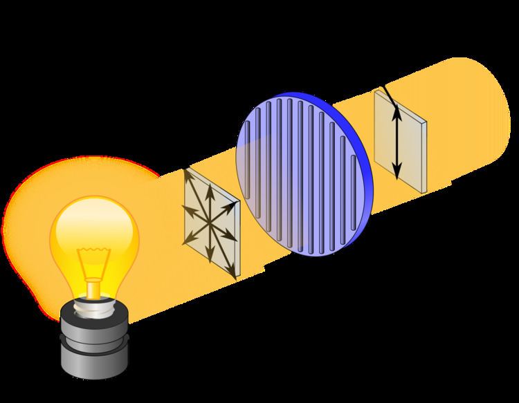
However, unpolarized light (such as the light from an incandescent light bulb) is different from any state like α | R ⟩ + β | L ⟩ (linear, circular, or elliptical polarization). Unlike linearly or elliptically polarized light, it passes through a polarizer with 50% intensity loss whatever the orientation of the polarizer; and unlike circularly polarized light, it cannot be made linearly polarized with any wave plate because randomly oriented polarization will emerge from a wave plate with random orientation. Indeed, unpolarized light cannot be described as any state of the form α | R ⟩ + β | L ⟩ in a definite sense. However, unpolarized light can be described with ensemble averages, e.g. that each photon is either | R ⟩ with 50% probability or | L ⟩ with 50% probability. The same behavior would occur if each photon was either vertically polarized with 50% probability or horizontally polarized with 50% probability.

Therefore, unpolarized light cannot be described by any pure state, but can be described as a statistical ensemble of pure states in at least two ways (the ensemble of half left and half right circularly polarized, or the ensemble of half vertically and half horizontally linearly polarized). These two ensembles are completely indistinguishable experimentally, and therefore they are considered the same mixed state. One of the advantages of the density matrix is that there is just one density matrix for each mixed state, whereas there are many statistical ensembles of pure states for each mixed state. Nevertheless, the density matrix contains all the information necessary to calculate any measurable property of the mixed state.

Where do mixed states come from? To answer that, consider how to generate unpolarized light. One way is to use a system in thermal equilibrium, a statistical mixture of enormous numbers of microstates, each with a certain probability (the Boltzmann factor), switching rapidly from one to the next due to thermal fluctuations. Thermal randomness explains why an incandescent light bulb, for example, emits unpolarized light. A second way to generate unpolarized light is to introduce uncertainty in the preparation of the system, for example, passing it through a birefringent crystal with a rough surface, so that slightly different parts of the beam acquire different polarizations. A third way to generate unpolarized light uses an EPR setup: A radioactive decay can emit two photons traveling in opposite directions, in the quantum state ( | R , L ⟩ + | L , R ⟩ ) / 2 . The two photons together are in a pure state, but if you only look at one of the photons and ignore the other, the photon behaves just like unpolarized light.

More generally, mixed states commonly arise from a statistical mixture of the starting state (such as in thermal equilibrium), from uncertainty in the preparation procedure (such as slightly different paths that a photon can travel), or from looking at a subsystem entangled with something else.

Mathematical description

The state vector | ψ ⟩ of a pure state completely determines the statistical behavior of a measurement. For concreteness, take an observable quantity, and let A be the associated observable operator that has a representation on the Hilbert space H of the quantum system. For any real-valued, analytical function F defined on the real numbers, suppose that F(A) is the result of applying F to the outcome of a measurement. The expectation value of F(A) is

Now consider a mixed state prepared by statistically combining two different pure states | ψ ⟩ and | ϕ ⟩ , with the associated probabilities p and 1 − p, respectively. The associated probabilities mean that the preparation process for the quantum system ends in the state | ψ ⟩ with probability p and in the state | ϕ ⟩ with probability 1 − p.

It is not hard to show that the statistical properties of the observable for the system prepared in such a mixed state are completely determined. However, there is no state vector | ξ ⟩ which determines this statistical behavior in the sense that the expectation value of F(A) is

Nevertheless, there is a unique operator ρ such that the expectation value of F(A) can be written as

where the operator ρ is the density operator of the mixed system. A simple calculation shows that the operator ρ for the above discussion is given by

For the above example of unpolarized light, the density operator is

Definition

For a finite-dimensional function space, the most general density operator is of the form

where the coefficients p_j are non-negative and add up to one. This represents a statistical mixture of pure states. If the given system is closed, then one can think of a mixed state as representing a single system with an uncertain preparation history, as explicitly detailed above; or we can regard the mixed state as representing an ensemble of systems, i.e. a large number of copies of the system in question, where p_j is the proportion of the ensemble being in the state | ψ j ⟩ . An ensemble is described by a pure state if every copy of the system in that ensemble is in the same state, i.e. it is a pure ensemble. If the system is not closed, however, then it is simply not correct to claim that it has some definite but unknown state vector, as the density operator may record physical entanglements to other systems.

Consider a quantum ensemble of size N with occupancy numbers n₁, n₂,...,n_k corresponding to the orthonormal states | 1 ⟩ , . . . , | k ⟩ , respectively, where n₁+...+n_k = N, and, thus, the coefficients p_j = n_j /N. For a pure ensemble, where all N particles are in state | i ⟩ , we have n_j = 0, for all j ≠ i, from which we recover the corresponding density operator ρ = | i ⟩ ⟨ i | . However, the density operator of a mixed state does not capture all the information about the ingredients that went into the mixture; in particular, the coefficients p_j and the kets ψ_j are not recoverable from the operator ρ without additional information. This non-uniqueness implies that different ensembles or mixtures may correspond to the same density operator. Such equivalent ensembles or mixtures cannot be distinguished by measurement of observables alone. This equivalence can be characterized precisely. Two ensembles ψ, ψ' define the same density operator if and only if there is a matrix U with

i.e., U is unitary and such that

This is simply a restatement of the following fact from linear algebra: for two square matrices M and N, M M^* = N N^* if and only if M = NU for some unitary U. (See square root of a matrix for more details.) Thus there is a unitary freedom in the ket mixture or ensemble that gives the same density operator. However, if the kets making up the mixture are restricted to be orthonormal, then the original probabilities p_j are recoverable as the eigenvalues of the density matrix.

In operator language, a density operator is a positive semidefinite, hermitian operator of trace 1 acting on the state space. A density operator describes a pure state if it is a rank one projection. Equivalently, a density operator ρ describes a pure state if and only if

i.e. the state is idempotent. This is true regardless of whether H is finite-dimensional or not.

Geometrically, when the state is not expressible as a convex combination of other states, it is a pure state. The family of mixed states is a convex set and a state is pure if it is an extremal point of that set.

It follows from the spectral theorem for compact self-adjoint operators that every mixed state is a countable convex combination of pure states. This representation is not unique. Furthermore, a theorem of Andrew Gleason states that certain functions defined on the family of projections and taking values in [0,1] (which can be regarded as quantum analogues of probability measures) are determined by unique mixed states. See quantum logic for more details.

Measurement

Let A be an observable of the system, and suppose the ensemble is in a mixed state such that each of the pure states | ψ j ⟩ occurs with probability p_j. Then the corresponding density operator is:

The expectation value of the measurement can be calculated by extending from the case of pure states (see Measurement in quantum mechanics):

where tr denotes trace. Moreover, if A has spectral resolution

where P i = | a i ⟩ ⟨ a i | , the corresponding density operator after the measurement is given by:

Note that the above density operator describes the full ensemble after measurement. The sub-ensemble for which the measurement result was the particular value a_i is described by the different density operator

This is true assuming that | a i ⟩ is the only eigenket (up to phase) with eigenvalue a_i; more generally, P_i in this expression would be replaced by the projection operator into the eigenspace corresponding to eigenvalue a_i.

Entropy

The von Neumann entropy S of a mixture can be expressed in terms of the eigenvalues of ρ or in terms of the trace and logarithm of the density operator ρ . Since ρ is a positive semi-definite operator, it has a spectral decomposition such that ρ = ∑ i λ i | φ i ⟩ ⟨ φ i | where | φ i ⟩ are orthonormal vectors, λ i > 0 and ∑ λ i = 1 . Then the entropy of a quantum system with density matrix ρ is

Also it can be shown that

when ρ i have orthogonal support, where H ( p ) is the Shannon entropy. This entropy can increase but never decrease with a projective measurement, however generalised measurements can decrease entropy. The entropy of a pure state is zero, while that of a proper mixture always greater than zero. Therefore, a pure state may be converted into a mixture by a measurement, but a proper mixture can never be converted into a pure state. Thus the act of measurement induces a fundamental irreversible change on the density matrix; this is analogous to the "collapse" of the state vector, or wavefunction collapse. Perhaps counterintuitively, the measurement actually decreases information by erasing quantum interference in the composite system—cf. quantum entanglement, einselection, and quantum decoherence.

(A subsystem of a larger system can be turned from a mixed to a pure state, but only by increasing the von Neumann entropy elsewhere in the system. This is analogous to how the entropy of an object can be lowered by putting it in a refrigerator: The air outside the refrigerator's heat-exchanger warms up, gaining even more entropy than was lost by the object in the refrigerator. See second law of thermodynamics. See Entropy in thermodynamics and information theory.)

The von Neumann equation for time evolution

Just as the Schrödinger equation describes how pure states evolve in time, the von Neumann equation (also known as the Liouville–von Neumann equation) describes how a density operator evolves in time (in fact, the two equations are equivalent, in the sense that either can be derived from the other.) The von Neumann equation dictates that

where the brackets denote a commutator.

Note that this equation only holds when the density operator is taken to be in the Schrödinger picture, even though this equation seems at first look to emulate the Heisenberg equation of motion in the Heisenberg picture, with a crucial sign difference:

where A ( H ) ( t ) is some Heisenberg picture operator; but in this picture the density matrix is not time-dependent, and the relative sign ensures that the time derivative of the expected value ⟨ A ⟩ comes out the same as in the Schrödinger picture.

Taking the density operator to be in the Schrödinger picture makes sense, since it is composed of 'Schrödinger' kets and bras evolved in time, as per the Schrödinger picture. If the Hamiltonian is time-independent, this differential equation can be easily solved to yield

For a more general Hamiltonian, if G ( t ) is the wavefunction propagator over some interval, then the time evolution of the density matrix over that same interval is given by

"Quantum Liouville", Moyal's equation

The density matrix operator may also be realized in phase space. Under the Wigner map, the density matrix transforms into the equivalent Wigner function,

The equation for the time-evolution of the Wigner function is then the Wigner-transform of the above von Neumann equation,

where H(q,p) is the Hamiltonian, and { { •,• } } is the Moyal bracket, the transform of the quantum commutator.

The evolution equation for the Wigner function is then analogous to that of its classical limit, the Liouville equation of classical physics. In the limit of vanishing Planck's constant ħ, W(q,p,t) reduces to the classical Liouville probability density function in phase space.

The classical Liouville equation can be solved using the method of characteristics for partial differential equations, the characteristic equations being Hamilton's equations. The Moyal equation in quantum mechanics similarly admits formal solutions in terms of quantum characteristics, predicated on the ∗−product of phase space, although, in actual practice, solution-seeking follows different methods.

Composite systems

The joint density matrix of a composite system of two systems A and B is described by ρ A B . Then the subsystems are described by their reduced density operator.

tr B is called partial trace over system B. If A and B are two distinct and independent systems then ρ A B = ρ A ⊗ ρ B which is a product state.

C*-algebraic formulation of states

It is now generally accepted that the description of quantum mechanics in which all self-adjoint operators represent observables is untenable. For this reason, observables are identified with elements of an abstract C*-algebra A (that is one without a distinguished representation as an algebra of operators) and states are positive linear functionals on A. However, by using the GNS construction, we can recover Hilbert spaces which realize A as a subalgebra of operators.

Geometrically, a pure state on a C*-algebra A is a state which is an extreme point of the set of all states on A. By properties of the GNS construction these states correspond to irreducible representations of A.

The states of the C*-algebra of compact operators K(H) correspond exactly to the density operators, and therefore the pure states of K(H) are exactly the pure states in the sense of quantum mechanics.

The C*-algebraic formulation can be seen to include both classical and quantum systems. When the system is classical, the algebra of observables become an abelian C*-algebra. In that case the states become probability measures, as noted in the introduction.