
Mean (not defined) | ||
 | ||
Parameters γ , σ > 0 {\displaystyle \gamma ,\sigma >0} Support x ∈ ( − ∞ , ∞ ) {\displaystyle x\in (-\infty ,\infty )} PDF ℜ [ w ( z ) ] σ 2 π , z = x + i γ σ 2 {\displaystyle {\frac {\Re [w(z)]}{\sigma {\sqrt {2\pi }}}},~~~z={\frac {x+i\gamma }{\sigma {\sqrt {2}}}}} CDF (complicated - see text) Median 0 {\displaystyle 0} | ||
In spectroscopy, the Voigt profile (named after Woldemar Voigt) is a line profile resulting from the convolution of two broadening mechanisms, one of which alone would produce a Gaussian profile (usually, as a result of the Doppler broadening), and the other would produce a Lorentzian profile. Voigt profiles are common in many branches of spectroscopy and diffraction. Due to the computational expense of the convolution operation, the Voigt profile is often approximated using a pseudo-Voigt profile.
Contents
- Properties
- Cumulative distribution function
- The width of the Voigt profile
- The uncentered Voigt profile
- Voigt functions
- Relation to Voigt profile
- Pseudo Voigt approximation
- References
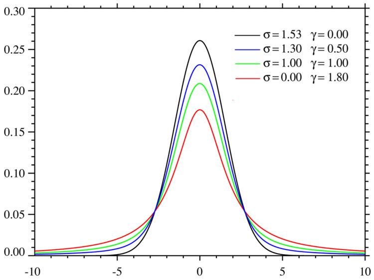
All normalized line profiles can be considered to be probability distributions. The Gaussian profile has a Gaussian, or normal, distribution and a Lorentzian profile has a Lorentz, or Cauchy, distribution. Without loss of generality, we can consider only centered profiles, which peak at zero. The Voigt profile is then a convolution of a Lorentz profile and a Gaussian profile:
where x is the shift from the line center,
and
The defining integral can be evaluated as:
where Re[w(z)] is the real part of the Faddeeva function evaluated for
Properties
The Voigt profile is normalized:
since it is a convolution of normalized profiles. The Lorentzian profile has no moments (other than the zeroth), and so the moment-generating function for the Cauchy distribution is not defined. It follows that the Voigt profile will not have a moment-generating function either, but the characteristic function for the Cauchy distribution is well defined, as is the characteristic function for the normal distribution. The characteristic function for the (centered) Voigt profile will then be the product of the two:
Since normal distributions and Cauchy distributions are stable distributions, they are each are closed under convolution (up to change of scale), and it follows that the Voigt distributions are also closed under convolution.
Cumulative distribution function
Using the above definition for z , the cumulative distribution function (CDF) can be found as follows:
Substituting the definition of the Faddeeva function (scaled complex error function) yields for the indefinite integral:
which may be solved to yield
where
The width of the Voigt profile
The full width at half maximum (FWHM) of the Voigt profile can be found from the widths of the associated Gaussian and Lorentzian widths. The FWHM of the Gaussian profile is
The FWHM of the Lorentzian profile is
Define Φ =
where
A better approximation with an accuracy of 0.02% is given by
This approximation is exactly correct for a pure Gaussian, but has an error of about 0.000305% for a pure Lorentzian profile.
The uncentered Voigt profile
If the Gaussian profile is centered at
The mode and median are both located at
Voigt functions
The Voigt functions U, V, and H (sometimes called the line broadening function) are defined by
where
erfc is the complementary error function, and w(z) is the Faddeeva function.
Relation to Voigt profile
with
and
Pseudo-Voigt approximation
The pseudo-Voigt profile (or pseudo-Voigt function) is an approximation of the Voigt profile V(x) using a linear combination of a Gaussian curve G(x) and a Lorentzian curve L(x) instead of their convolution.
The pseudo-Voigt function is often used for calculations of experimental spectral line shapes.
The mathematical definition of the normalized pseudo-Voigt profile is given by
There are several possible choices for the
where