Viterbi algorithm

History

The Viterbi algorithm is named after Andrew Viterbi, who proposed it in 1967 as a decoding algorithm for convolutional codes over noisy digital communication links. It has, however, a history of multiple invention, with at least seven independent discoveries, including those by Viterbi, Needleman and Wunsch, and Wagner and Fischer.

"Viterbi path" and "Viterbi algorithm" have become standard terms for the application of dynamic programming algorithms to maximization problems involving probabilities. For example, in statistical parsing a dynamic programming algorithm can be used to discover the single most likely context-free derivation (parse) of a string, which is commonly called the "Viterbi parse".

Extensions

A generalization of the Viterbi algorithm, termed the max-sum algorithm (or max-product algorithm) can be used to find the most likely assignment of all or some subset of latent variables in a large number of graphical models, e.g. Bayesian networks, Markov random fields and conditional random fields. The latent variables need in general to be connected in a way somewhat similar to an HMM, with a limited number of connections between variables and some type of linear structure among the variables. The general algorithm involves message passing and is substantially similar to the belief propagation algorithm (which is the generalization of the forward-backward algorithm).

With the algorithm called iterative Viterbi decoding one can find the subsequence of an observation that matches best (on average) to a given hidden Markov model. This algorithm is proposed by Qi Wang et al. to deal with turbo code. Iterative Viterbi decoding works by iteratively invoking a modified Viterbi algorithm, reestimating the score for a filler until convergence.

An alternative algorithm, the Lazy Viterbi algorithm, has been proposed recently. For many codes of practical interest, under reasonable noise conditions, the lazy decoder (using Lazy Viterbi algorithm) is much faster than the original Viterbi decoder (using Viterbi algorithm). This algorithm works by not expanding any nodes until it really needs to, and usually manages to get away with doing a lot less work (in software) than the ordinary Viterbi algorithm for the same result - however, it is not so easy to parallelize in hardware.

Pseudocode

This algorithm generates a path X = ( x 1 , x 2 , … , x T ) , which is a sequence of states x n ∈ S = { s 1 , s 2 , … , s K } that generate the observations Y = ( y 1 , y 2 , … , y T ) .

Two 2-dimensional tables of size are constructed:

Each element T 1 [ i , j ] of T 1 stores the probability of the most likely path so far X ^ = ( x ^ 1 , x ^ 2 , … , x ^ j ) with x ^ j = s i that generates Y = ( y 1 , y 2 , … , y j ) .

Each element T 2 [ i , j ] of T 2 stores x ^ j − 1 of the most likely path so far X ^ = ( x ^ 1 , x ^ 2 , … , x ^ j − 1 , x ^ j = s i ) for ∀ j , 2 ≤ j ≤ T

The table entries T 1 [ i , j ] , T 2 [ i , j ] are filled by increasing order of K ⋅ j + i .

T 1 [ i , j ] = max k ( T 1 [ k , j − 1 ] ⋅ A k i ) ⋅ B i y j , and T 2 [ i , j ] = arg ⁡ max k ( T 1 [ k , j − 1 ] ⋅ A k i )

Note that B i y j does not need to appear in the latter expression, as it's non-negative and independent of k and thus does not affect the argmax.

INPUT

The observation space O = { o 1 , o 2 , … , o N }

the state space S = { s 1 , s 2 , … , s K }

an array of initial probabilities Π = ( π 1 , π 2 , … , π K ) such that π i stores the probability that x 1 == s i

a sequence of observations Y = ( y 1 , y 2 , … , y T ) such that y t == i if the observation at time t is o i

transition matrix A of size K ⋅ K such that A i j stores the transition probability of transiting from state s i to state s j

emission matrix B of size K ⋅ N such that B i j stores the probability of observing o j from state s i

OUTPUT

The most likely hidden state sequence X = ( x 1 , x 2 , … , x T )

function VITERBI ( O , S , Π , Y , A , B ) : X for each state i ∈ { 1 , 2 , … , K } do T₁[i,1] ← π_i·B_iy1 T₂[i,1] ← 0 end for for each observation i ∈ { 2 , 3 , … , T } do for each state j ∈ { 1 , 2 , … , K } do T 1 [ j , i ] ← B j y i ⋅ max k ( T 1 [ k , i − 1 ] ⋅ A k j ) T 2 [ j , i ] ← arg ⁡ max k ( T 1 [ k , i − 1 ] ⋅ A k j ) end for end for z T ← arg ⁡ max k ( T 1 [ k , T ] ) x_T ← s_zT for i ← T,T-1,...,2 do z_i-1 ← T₂[z_i,i] x_i-1 ← s_zi-1 end for return X end function

EXPLANATION

Suppose we are given a hidden Markov model (HMM) with state space S , initial probabilities π i of being in state i and transition probabilities a i , j of transitioning from state i to state j . Say we observe outputs y 1 , … , y T . The most likely state sequence x 1 , … , x T that produces the observations is given by the recurrence relations:

V 1 , k = P ( y 1   |   k ) ⋅ π k V t , k = max x ∈ S ( P ( y t   |   k ) ⋅ a x , k ⋅ V t − 1 , x )

Here V t , k is the probability of the most probable state sequence P ( x 1 , … , x T , y 1 , … , y T ) responsible for the first t observations that have k as its final state. The Viterbi path can be retrieved by saving back pointers that remember which state x was used in the second equation. Let P t r ( k , t ) be the function that returns the value of x used to compute V t , k if t > 1 , or k if t = 1 . Then:

x T = arg ⁡ max x ∈ S ( V T , x ) x t − 1 = P t r ( x t , t )

Here we're using the standard definition of arg max.
The complexity of this algorithm is O ( T × | S | 2 ) .

Example

Consider a village where all villagers are either healthy or have a fever and only the village doctor can determine whether each has a fever. The doctor diagnoses fever by asking patients how they feel. The villagers may only answer that they feel normal, dizzy, or cold.

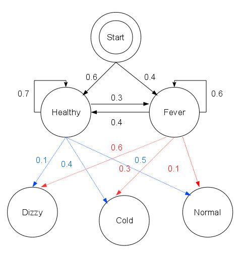
The doctor believes that the health condition of his patients operate as a discrete Markov chain. There are two states, "Healthy" and "Fever", but the doctor cannot observe them directly; they are hidden from him. On each day, there is a certain chance that the patient will tell the doctor he/she is "normal", "cold", or "dizzy", depending on her health condition.

The observations (normal, cold, dizzy) along with a hidden state (healthy, fever) form a hidden Markov model (HMM), and can be represented as follows in the Python programming language:

In this piece of code, start_probability represents the doctor's belief about which state the HMM is in when the patient first visits (all he knows is that the patient tends to be healthy). The particular probability distribution used here is not the equilibrium one, which is (given the transition probabilities) approximately {'Healthy': 0.57, 'Fever': 0.43}. The transition_probability represents the change of the health condition in the underlying Markov chain. In this example, there is only a 30% chance that tomorrow the patient will have a fever if he is healthy today. The emission_probability represents how likely the patient is to feel on each day. If he is healthy, there is a 50% chance that he feels normal; if he has a fever, there is a 60% chance that he feels dizzy.

The patient visits three days in a row and the doctor discovers that on the first day she feels normal, on the second day she feels cold, on the third day she feels dizzy. The doctor has a question: what is the most likely sequence of health conditions of the patient that would explain these observations? This is answered by the Viterbi algorithm.

The function viterbi takes the following arguments: obs is the sequence of observations, e.g. ['normal', 'cold', 'dizzy']; states is the set of hidden states; start_p is the start probability; trans_p are the transition probabilities; and emit_p are the emission probabilities. For simplicity of code, we assume that the observation sequence obs is non-empty and that trans_p[i][j] and emit_p[i][j] is defined for all states i,j.

In the running example, the forward/Viterbi algorithm is used as follows:

The output of the script is

This reveals that the observations ['normal', 'cold', 'dizzy'] were most likely generated by states ['Healthy', 'Healthy', 'Fever']. In other words, given the observed activities, the patient was most likely to have been healthy both on the first day when she felt normal as well as on the second day when she felt cold, and then she contracted a fever the third day.

The operation of Viterbi's algorithm can be visualized by means of a trellis diagram. The Viterbi path is essentially the shortest path through this trellis. The trellis for the clinic example is shown below; the corresponding Viterbi path is in bold:

Implementations

Susa signal processing framework provides the C++ implementation for Forward error correction codes and channel equalization here.

C#

Java

Java 8

Perl

Prolog

Haskell

Go

SFIHMM includes code for Viterbi decoding.