Needleman–Wunsch algorithm

Beginner's How-To Guide

This algorithm can be used for any two strings. This guide will use two small DNA sequences as examples as shown in the diagram:

GCATGCU GATTACA

Construct Grid

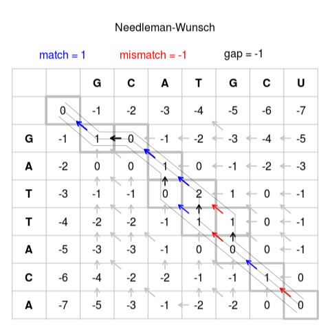
First construct a grid such as one shown in Figure 1 above. Start the first string in the top of the Third column and start the other string at the start of the 3rd row. Fill out the rest of the column and row headers as in Figure 1. There should be no numbers in the grid yet.

Choose Scoring System

Next we need to decide how to score how each individual pair of letters match up. Just by looking at our two strings you may be able to see one possible best alignment:

GCATG-CU G-ATTACA

We can see that letters may match, mismatch, be deleted or inserted (indel):

Match: The two letters are the same

Mismatch: The two letters are differential

Indel (INsertion or DELetion) : One letter aligns to a gap in the other string.

There are various ways to score these three scenarios. These have been outlined in the Scoring Systems section below. For now we will use the simple system used by Needleman and Wunsch; matches are given +1, mismatches are given -1 and indels are given -1.

Fill in the Table

Start with a zero in the second row, second column. Move through the cells row by row, calculating the score for each cell. The score is calculated as the best possible score (i.e. highest) from existing scores to the left, top or top-left (diagonal). When a score is calculated from the top, or from the left this represents an indel in our alignment. When we calculate scores from the diagonal this represents the alignment of the two letters the resulting cell matches to. Given there is no 'top' or 'top-left' cells for the second row we can only add from the existing cell to the left. Hence we add -1 for each shift to the right as this represents an indel from the previous score. This results in the first row being 0, -1, -2, -3, -4, -5, -6, -7. The same applies to the second column as we only have existing scores above. Thus we have:

The first case with existing scores in all 3 directions is the intersection of our first letters (in this case G and G). The surrounding cells are below:

As for all following cells, we have three options here. Firstly the score could be calculated from the existing score on top. In this case we would add -1 as this represents an indel, resulting in a total of -2. The same applies if we calculate from the existing score to the left. Calculating from the diagonal (top-left) existing score represents two letters aligned together. If the letters are the same this is a match, otherwise it is a mismatch. In this case the bases match and so we add +1. So we have -2, -2 and +1 as possible scores to choose from. The diagonal score is the best score so we give the cell a score of 1. We also need to keep track of where the score came from, shown as an arrow in the completed figure. Below shows samples from our example where the best score comes from the left and top cells respectively.

In some cells 2 or even all 3 of the originating cells may result in equal best scores such as this segment of figure x:

Here we can see that the score of zero is obtained both from the top cell and the top-left cell (both are 1 – 1=0). This represents the branching of two equally good alignments. In this scenario we need to fill in arrows to both cells. Follow this procedure for all the remaining cells until the table is filled.

The score in the last cell (bottom right) represents the alignment score for the best alignment.

Trace Arrows back to origin

Note that there are multiple equally 'best' alignments, here we show just one.

Follow the arrows back to the original cell to obtain the path for the best alignment. Then follow the path from start to finish to construct the alignment based on these rules

A diagonal arrow represents a match or mismatch, either way this means each letter corresponds to another letter. For example, the first arrow represents:

Nothing --> G Nothing --> G

If there is a horizontal arrow there will be two columns for one row in the alignment and hence a gap in the side string. This gap is after the letter in the row. For example, the second arrow represents:

G --> GC G --> G-

If there is a vertical arrow there will be two rows for one column in the alignment and hence a gap in the top string. This gap is after the letter in the column. For example, the fourth arrow represents:

GCA --> GCA- G-A --> G-AT

Note how there are multiple 'fourth' arrows to choose from, these represent branching of the alignments. If these branches return the last cell with the same score then they are equally viable alignments

Following these rules one possible alignment is constructed as follows:

G → GC → GCA → GCA- → GCA-T → GCA-TG → GCA-TGC → GCA-TGCU G → G- → G-A → G-AT → G-ATT → G-ATTA → G-ATTAC → G-ATTACA

Basic scoring schemes

The simplest scoring schemes simply give a value for each match, mismatch and indel. The step-by-step guide above uses match = 1, mismatch = -1, indel = -1. Thus the lower the alignment score the larger the edit distance, for this scoring system we want a high score. Another scoring system might be:

Match = 0

Indel = 1

Mismatch = 1

For this system the alignment score will represent the edit distance between the two strings. Different scoring systems can be devised for different situations, for example if gaps are considered very bad for your alignment you may use a scoring system that penalises gaps heavily, such as:

Match = 0

Mismatch = 1

Indel = 10

Similarity Matrix

More complicated scoring systems attribute values not only for the type of alteration, but also for the letters that are involved. For example, a match between A and A may be given 1, but a match between T and T may be given 4. Here (assuming the first scoring system) more importance is given to the Ts matching than the As, i.e. we think the Ts matching is more significant to our alignment. This weighting based on letters also applies to mismatches. In order to represent all the possible combinations of letters and their resulting scores we use a similarity matrix. The similarity matrix for the most basic system is represented as:

Each score represents a switch from one of the letters the cell matches to the other. Hence this represents all possible matches and deletions (for an alphabet of ACGT). Note all the matches go along the diagonal, also not all the table needs to be filled, only this triangle because the scores are reciprocal.= (Score for A → C = Score for C → A). If we implement our T-T = 4 from above we get:

Different scoring matrices have been statistically constructed which give weight to different actions appropriate to a particular scenario. Having weighted scoring matrices is particularly important in protein sequence alignment due to the varying frequency of the different amino acids. There are two broad families of scoring matrices, each with further alterations for specific scenarios:

PAM

BLOSUM

Gap penalty

When aligning sequences there are often gaps (i.e. indels), sometimes large ones. Biologically, a large gap is more likely to occur as one large deletion as opposed to multiple single deletions. Hence we should score two small indels to be worse than one large one. The simple and common way to do this is via a large gap-start score for a new indel and a smaller gap-extension score for every letter which extends the indel. For example, new-indel may cost -5 and extend-indel may cost -1. In this way an alignment such as:

GAAAAAAT G--A-A-T

which has multiple equal alignments, some with multiple small alignments will now align as:

GAAAAAAT GAA----T

or any alignment with a 4 long gap in preference over multiple small gaps.

Advanced presentation of algorithm

Scores for aligned characters are specified by a similarity matrix. Here, S(a, b) is the similarity of characters a and b. It uses a linear gap penalty, here called d.

For example, if the similarity matrix was

then the alignment:

AGACTAGTTAC CGA---GACGT

with a gap penalty of -5, would have the following score:

S(A,C) + S(G,G) + S(A,A) + (3 × d) + S(G,G) + S(T,A) + S(T,C) + S(A,G) + S(C,T) = -3 + 7 + 10 - (3 × 5) + 7 + (-4) + 0 + (-1) + 0 = 1

To find the alignment with the highest score, a two-dimensional array (or matrix) F is allocated. The entry in row i and column j is denoted here by F i j . There is one row for each character in sequence A, and one column for each character in sequence B. Thus, if we are aligning sequences of sizes n and m, the amount of memory used is in O ( n m ) . Hirschberg's algorithm only holds a subset of the array in memory and uses Θ ( min { n , m } ) space, but is otherwise similar to Needleman-Wunsch (and still requires O ( n m ) time).

As the algorithm progresses, the F i j will be assigned to be the optimal score for the alignment of the first i = 0 , … , n characters in A and the first j = 0 , … , m characters in B. The principle of optimality is then applied as follows:

Basis:

F 0 j = d ∗ j F i 0 = d ∗ i

Recursion, based on the principle of optimality:

F i j = max ( F i − 1 , j − 1 + S ( A i , B j ) , F i , j − 1 + d , F i − 1 , j + d )

The pseudo-code for the algorithm to compute the F matrix therefore looks like this:

for i=0 to length(A) F(i,0) ← d*i for j=0 to length(B) F(0,j) ← d*j for i=1 to length(A) for j=1 to length(B) { Match ← F(i-1,j-1) + S(A_i, B_j) Delete ← F(i-1, j) + d Insert ← F(i, j-1) + d F(i,j) ← max(Match, Insert, Delete) }

Once the F matrix is computed, the entry F n m gives the maximum score among all possible alignments. To compute an alignment that actually gives this score, you start from the bottom right cell, and compare the value with the three possible sources (Match, Insert, and Delete above) to see which it came from. If Match, then A i and B j are aligned, if Delete, then A i is aligned with a gap, and if Insert, then B j is aligned with a gap. (In general, more than one choice may have the same value, leading to alternative optimal alignments.)

AlignmentA ← "" AlignmentB ← "" i ← length(A) j ← length(B) while (i > 0 or j > 0) { if (i > 0 and j > 0 and F(i,j) == F(i-1,j-1) + S(A_i, B_j)) { AlignmentA ← A_i + AlignmentA AlignmentB ← B_j + AlignmentB i ← i - 1 j ← j - 1 } else if (i > 0 and F(i,j) == F(i-1,j) + d) { AlignmentA ← A_i + AlignmentA AlignmentB ← "-" + AlignmentB i ← i - 1 } else { AlignmentA ← "-" + AlignmentA AlignmentB ← B_j + AlignmentB j ← j - 1 } }

Global alignment tools using the Needleman-Wunsch algorithm

EMBOSS Needle and EMBOSS Stretcher Global Alignment Tools

Needleman-Wunsch alignment for two nucleotide sequences

MathWorks - Globally align two sequences using Needleman-Wunsch algorithm

Computer stereo vision

Stereo matching is an essential step in the process of 3D reconstruction from a pair of stereo images. When images have been rectified, an analogy can be drawn between aligning nucleotide/protein sequences and matching pixels belonging to scan lines, since both tasks aim at establishing optimal correspondence between two strings of characters. Indeed, the ‘right’ image of a stereo pair can be seen as a mutated version of the ‘left’ image: noise and individual camera sensitivity alter pixel values (i.e. character substitutions); and different view angle reveals previously occluded data and introduces new occlusions (i.e. insertion and deletion of characters). As consequence, minor modifications of the Needleman–Wunsch algorithm make it suitable for stereo matching. Although performances in terms of accuracy are not state-of-the-art, the relative simplicity of the algorithm allows its implementation on embedded systems.

Although in many applications image rectification can be performed, e.g. by camera resectioning or calibration, it is sometimes impossible or impractical since the computational cost of accurate rectification models prohibit their usage in real-time applications. Moreover, none of these models is suitable when a camera lens displays unexpected distortions, such as those generated by raindrops, weatherproof covers or dust. By extending the Needleman–Wunsch algorithm, a line in the ‘left’ image can be associated to a curve in the ‘right’ image by finding the alignment with the highest score in a three-dimensional array (or matrix). Experiments demonstrated that such extension allows dense pixel matching between unrectified and/or distorted images.