Toroidal coordinates - Alchetron, The Free Social Encyclopedia

Toroidal coordinates are a three-dimensional orthogonal coordinate system that results from rotating the two-dimensional bipolar coordinate system about the axis that separates its two foci. Thus, the two foci F 1 and F 2 in bipolar coordinates become a ring of radius a in the x y plane of the toroidal coordinate system; the z -axis is the axis of rotation. The focal ring is also known as the reference circle.

Definition

The most common definition of toroidal coordinates ( σ , τ , ϕ ) is

x = a sinh ⁡ τ cosh ⁡ τ − cos ⁡ σ cos ⁡ ϕ y = a sinh ⁡ τ cosh ⁡ τ − cos ⁡ σ sin ⁡ ϕ z = a sin ⁡ σ cosh ⁡ τ − cos ⁡ σ

where the σ coordinate of a point P equals the angle F 1 P F 2 and the τ coordinate equals the natural logarithm of the ratio of the distances d 1 and d 2 to opposite sides of the focal ring

τ = ln ⁡ d 1 d 2 .

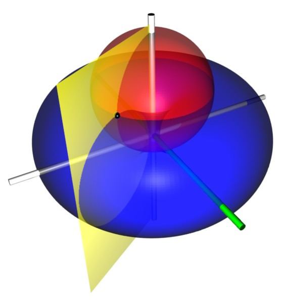
The coordinate ranges are − π < σ ≤ π and τ ≥ 0 and 0 ≤ ϕ < 2 π .

Coordinate surfaces

Surfaces of constant σ correspond to spheres of different radii

( x 2 + y 2 ) + ( z − a cot ⁡ σ ) 2 = a 2 sin 2 ⁡ σ

that all pass through the focal ring but are not concentric. The surfaces of constant τ are non-intersecting tori of different radii

z 2 + ( x 2 + y 2 − a coth ⁡ τ ) 2 = a 2 sinh 2 ⁡ τ

that surround the focal ring. The centers of the constant- σ spheres lie along the z -axis, whereas the constant- τ tori are centered in the x y plane.

Inverse transformation

The (σ, τ, φ) coordinates may be calculated from the Cartesian coordinates (x, y, z) as follows. The azimuthal angle φ is given by the formula

tan ⁡ ϕ = y x

The cylindrical radius ρ of the point P is given by

ρ 2 = x 2 + y 2

and its distances to the foci in the plane defined by φ is given by

d 1 2 = ( ρ + a ) 2 + z 2 d 2 2 = ( ρ − a ) 2 + z 2

The coordinate τ equals the natural logarithm of the focal distances

τ = ln ⁡ d 1 d 2

whereas the coordinate σ equals the angle between the rays to the foci, which may be determined from the law of cosines

cos ⁡ σ = − 4 a 2 − d 1 2 − d 2 2 2 d 1 d 2

where the sign of σ is determined by whether the coordinate surface sphere is above or below the x-y plane.

Scale factors

The scale factors for the toroidal coordinates σ and τ are equal

h σ = h τ = a cosh ⁡ τ − cos ⁡ σ

whereas the azimuthal scale factor equals

h ϕ = a sinh ⁡ τ cosh ⁡ τ − cos ⁡ σ

Thus, the infinitesimal volume element equals

d V = a 3 sinh ⁡ τ ( cosh ⁡ τ − cos ⁡ σ ) 3 d σ d τ d ϕ

and the Laplacian is given by

∇ 2 Φ = ( cosh ⁡ τ − cos ⁡ σ ) 3 a 2 sinh ⁡ τ [ sinh ⁡ τ ∂ ∂ σ ( 1 cosh ⁡ τ − cos ⁡ σ ∂ Φ ∂ σ ) + ∂ ∂ τ ( sinh ⁡ τ cosh ⁡ τ − cos ⁡ σ ∂ Φ ∂ τ ) + 1 sinh ⁡ τ ( cosh ⁡ τ − cos ⁡ σ ) ∂ 2 Φ ∂ ϕ 2 ]

Other differential operators such as ∇ ⋅ F and ∇ × F can be expressed in the coordinates ( σ , τ , ϕ ) by substituting the scale factors into the general formulae found in orthogonal coordinates.

Standard separation

The 3-variable Laplace equation

∇ 2 Φ = 0

admits solution via separation of variables in toroidal coordinates. Making the substitution

Φ = U cosh ⁡ τ − cos ⁡ σ

A separable equation is then obtained. A particular solution obtained by separation of variables is:

Φ = cosh ⁡ τ − cos ⁡ σ S ν ( σ ) T μ ν ( τ ) V μ ( ϕ )

where each function is a linear combination of:

S ν ( σ ) = e i ν σ a n d e − i ν σ T μ ν ( τ ) = P ν − 1 / 2 μ ( cosh ⁡ τ ) a n d Q ν − 1 / 2 μ ( cosh ⁡ τ ) V μ ( ϕ ) = e i μ ϕ a n d e − i μ ϕ

Where P and Q are associated Legendre functions of the first and second kind. These Legendre functions are often referred to as toroidal harmonics.

Toroidal harmonics have many interesting properties. If you make a variable substitution 1 < z = cosh ⁡ η then, for instance, with vanishing order (the convention is to not write the order when it vanishes) and n = 0

Q − 1 2 ( z ) = 2 1 + z K ( 2 1 + z )

and

P − 1 2 ( z ) = 2 π 2 1 + z K ( z − 1 z + 1 )

where K and E are the complete elliptic integrals of the first and second kind respectively. The rest of the toroidal harmonics can be obtained, for instance, in terms of the complete elliptic integrals, by using recurrence relations for associated Legendre functions.

The classic applications of toroidal coordinates are in solving partial differential equations, e.g., Laplace's equation for which toroidal coordinates allow a separation of variables or the Helmholtz equation, for which toroidal coordinates do not allow a separation of variables. Typical examples would be the electric potential and electric field of a conducting torus, or in the degenerate case, an electric current-ring (Hulme 1982).

An alternative separation

Alternatively, a different substitution may be made (Andrews 2006)

Φ = U ρ

where

ρ = x 2 + y 2 = a sinh ⁡ τ cosh ⁡ τ − cos ⁡ σ .

Again, a separable equation is obtained. A particular solution obtained by separation of variables is then:

Φ = a ρ S ν ( σ ) T μ ν ( τ ) V μ ( ϕ )

where each function is a linear combination of:

S ν ( σ ) = e i ν σ a n d e − i ν σ T μ ν ( τ ) = P μ − 1 / 2 ν ( coth ⁡ τ ) a n d Q μ − 1 / 2 ν ( coth ⁡ τ ) V μ ( ϕ ) = e i μ ϕ a n d e − i μ ϕ .

Note that although the toroidal harmonics are used again for the T function, the argument is coth ⁡ τ rather than cosh ⁡ τ and the μ and ν indices are exchanged. This method is useful for situations in which the boundary conditions are independent of the spherical angle θ , such as the charged ring, an infinite half plane, or two parallel planes. For identities relating the toroidal harmonics with argument hyperbolic cosine with those of argument hyperbolic cotangent, see the Whipple formulae.

References

Toroidal coordinates Wikipedia

(Text) CC BY-SA

Contents