
 | ||
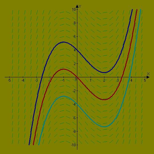
The solutions of a first-order differential equation of a scalar function y(x) can be drawn in a 2-dimenional space with the x in horizontal and y in vertical direction. Possible solutions are functions y(x) drawn as solid curves. Somtimes it is too cumbersome solving the differential equation analytically. Then one can still draw the tangents of the function curves e.g on a regular grid. The tangents are touching the functions at the grid points. However, the direction field is rather agnostic about chaotic aspects of the differential equation.
Contents
Standard case
The slope field can be defined for the following type of differential equations
which can be interpreted geometrically as giving the slope of the tangent to the graph of the differential equation's solution (integral curve) at each point (x, y) as a function of the point coordinates.
It can be viewed as a creative way to plot a real-valued function of two real variables
An isocline (a series of lines with the same slope) is often used to supplement the slope field. In an equation of the form
General case of a system of differential equations
Given a system of differential equations,
the slope field is an array of slope marks in the phase space (in any number of dimensions depending on the number of relevant variables; for example, two in the case of a first-order linear ODE, as seen to the right). Each slope mark is centered at a point
The number, position, and length of the slope marks can be arbitrary. The positions are usually chosen such that the points
General application
With computers, complicated slope fields can be quickly made without tedium, and so an only recently practical application is to use them merely to get the feel for what a solution should be before an explicit general solution is sought. Of course, computers can also just solve for one, if it exists.
If there is no explicit general solution, computers can use slope fields (even if they aren’t shown) to numerically find graphical solutions. Examples of such routines are Euler's method, or better, the Runge–Kutta methods.
Software for plotting slope fields
Different software packages can plot slope fields.