Simplex

Examples

A 0-simplex is a point.

A 1-simplex is a line segment.

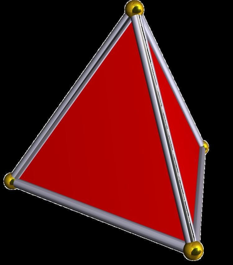
A 2-simplex is a triangle.

A 3-simplex is a tetrahedron.

A 4-simplex is a 5-cell.

Elements

The convex hull of any nonempty subset of the n+1 points that define an n-simplex is called a face of the simplex. Faces are simplices themselves. In particular, the convex hull of a subset of size m+1 (of the n+1 defining points) is an m-simplex, called an m-face of the n-simplex. The 0-faces (i.e., the defining points themselves as sets of size 1) are called the vertices (singular: vertex), the 1-faces are called the edges, the (n − 1)-faces are called the facets, and the sole n-face is the whole n-simplex itself. In general, the number of m-faces is equal to the binomial coefficient ( n + 1 m + 1 ) . Consequently, the number of m-faces of an n-simplex may be found in column (m + 1) of row (n + 1) of Pascal's triangle. A simplex A is a coface of a simplex B if B is a face of A. Face and facet can have different meanings when describing types of simplices in a simplicial complex; see simplical complex for more detail.

The regular simplex family is the first of three regular polytope families, labeled by Coxeter as α_n, the other two being the cross-polytope family, labeled as β_n, and the hypercubes, labeled as γ_n. A fourth family, the infinite tessellation of hypercubes, he labeled as δ_n.

The number of 1-faces (edges) of the n-simplex is the n-th triangle number, the number of 2-faces of the n-simplex is the (n-1)th tetrahedron number, the number of 3-faces of the n-simplex is the (n-2)th 5-cell number, and so on.

An (n+1)-simplex can be constructed as a join (∨ operator) of an n-simplex and a point, ( ). An (m+n+1)-simplex can be constructed as a join of an m-simplex and an n-simplex. The two simplices are oriented to be completely normal from each other, with translation in a direction orthogonal to both of them. A 1-simplex is a joint of two points: ( )∨( ) = 2.( ). A general 2-simplex (scalene triangle) is the join of 3 points: ( )∨( )∨( ). An isosceles triangle is the join of a 1-simplex and a point: { }∨( ). An equilateral triangle is 3.( ) or {3}. A general 3-simplex is the join of 4 points: ( )∨( )∨( )∨( ). A 3-simplex with mirror symmetry can be expressed as the join of an edge and 2 points: { }∨( )∨( ). A 3-simplex with triangular symmetry can be expressed as the join of an equilateral triangle and 1 point: 3.( )∨( ) or {3}∨( ). A regular tetrahedron is 4.( ) or {3,3} and so on.

In some conventions, the empty set is defined to be a (−1)-simplex. The definition of the simplex above still makes sense if n = −1. This convention is more common in applications to algebraic topology (such as simplicial homology) than to the study of polytopes.

Symmetric graphs of regular simplices

These Petrie polygons (skew orthogonal projections) show all the vertices of the regular simplex on a circle, and all vertex pairs connected by edges.

The standard simplex

The standard n-simplex (or unit n-simplex) is the subset of Rⁿ⁺¹ given by

Δ n = { ( t 0 , ⋯ , t n ) ∈ R n + 1 ∣ ∑ i = 0 n t i = 1  and  t i ≥ 0  for all  i }

The simplex Δⁿ lies in the affine hyperplane obtained by removing the restriction t_i ≥ 0 in the above definition.

The n+1 vertices of the standard n-simplex are the points e_i ∈ Rⁿ⁺¹, where

e₀ = (1, 0, 0, ..., 0), e₁ = (0, 1, 0, ..., 0), ⋮ e_n = (0, 0, 0, ..., 1).

There is a canonical map from the standard n-simplex to an arbitrary n-simplex with vertices (v₀, …, v_n) given by

( t 0 , ⋯ , t n ) ↦ ∑ i = 0 n t i v i

The coefficients t_i are called the barycentric coordinates of a point in the n-simplex. Such a general simplex is often called an affine n-simplex, to emphasize that the canonical map is an affine transformation. It is also sometimes called an oriented affine n-simplex to emphasize that the canonical map may be orientation preserving or reversing.

More generally, there is a canonical map from the standard ( n − 1 ) -simplex (with n vertices) onto any polytope with n vertices, given by the same equation (modifying indexing):

( t 1 , ⋯ , t n ) ↦ ∑ i = 1 n t i v i

These are known as generalized barycentric coordinates, and express every polytope as the image of a simplex: Δ n − 1 ↠ P .

Examples

Δ⁰ is the point 1 in R¹.

Δ¹ is the line segment joining (1,0) and (0,1) in R².

Δ² is the equilateral triangle with vertices (1,0,0), (0,1,0) and (0,0,1) in R³.

Δ³ is the regular tetrahedron with vertices (1,0,0,0), (0,1,0,0), (0,0,1,0) and (0,0,0,1) in R⁴.

Increasing coordinates

An alternative coordinate system is given by taking the indefinite sum:

s 0 = 0 s 1 = s 0 + t 0 = t 0 s 2 = s 1 + t 1 = t 0 + t 1 s 3 = s 2 + t 2 = t 0 + t 1 + t 2 … s n = s n − 1 + t n − 1 = t 0 + t 1 + ⋯ + t n − 1 s n + 1 = s n + t n = t 0 + t 1 + ⋯ + t n = 1

This yields the alternative presentation by order, namely as nondecreasing n-tuples between 0 and 1:

Δ ∗ n = { ( s 1 , ⋯ , s n ) ∈ R n ∣ 0 = s 0 ≤ s 1 ≤ s 2 ≤ ⋯ ≤ s n ≤ s n + 1 = 1 } .

Geometrically, this is an n-dimensional subset of R n (maximal dimension, codimension 0) rather than of R n + 1 (codimension 1). The facets, which on the standard simplex correspond to one coordinate vanishing, t i = 0 , here correspond to successive coordinates being equal, s i = s i + 1 , while the interior corresponds to the inequalities becoming strict (increasing sequences).

A key distinction between these presentations is the behavior under permuting coordinates – the standard simplex is stabilized by permuting coordinates, while permuting elements of the "ordered simplex" do not leave it invariant, as permuting an ordered sequence generally makes it unordered. Indeed, the ordered simplex is a (closed) fundamental domain for the action of the symmetric group on the n-cube, meaning that the orbit of the ordered simplex under the n! elements of the symmetric group divides the n-cube into n ! mostly disjoint simplices (disjoint except for boundaries), showing that this simplex has volume 1 / n ! Alternatively, the volume can be computed by an iterated integral, whose successive integrands are 1 , x , x 2 / 2 , x 3 / 3 ! , … , x n / n !

A further property of this presentation is that it uses the order but not addition, and thus can be defined in any dimension over any ordered set, and for example can be used to define an infinite-dimensional simplex without issues of convergence of sums.

Projection onto the standard simplex

Especially in numerical applications of probability theory a projection onto the standard simplex is of interest. Given ( p i ) i with possibly negative entries, the closest point ( t i ) i on the simplex has coordinates

t i = max { p i + Δ , 0 } ,

where Δ is chosen such that ∑ i max { p i + Δ , 0 } = 1.

Δ can be easily calculated from sorting p i . The sorting approach takes O ( n log ⁡ n ) complexity, which can be improved to O ( n ) complexity via median-finding algorithms. Projecting onto the simplex is computationally similar to projecting onto the ℓ 1 ball.

Corner of cube

Finally, a simple variant is to replace "summing to 1" with "summing to at most 1"; this raises the dimension by 1, so to simplify notation, the indexing changes:

Δ c n = { ( t 1 , ⋯ , t n ) ∈ R n ∣ ∑ i = 1 n t i ≤ 1  and  t i ≥ 0  for all  i } .

This yields an n-simplex as a corner of the n-cube, and is a standard orthogonal simplex. This is the simplex used in the simplex method, which is based at the origin, and locally models a vertex on a polytope with n facets.

Cartesian coordinates for regular n-dimensional simplex in Rn

The coordinates of the vertices of a regular n-dimensional simplex can be obtained from these two properties,

1. For a regular simplex, the distances of its vertices to its center are equal.
2. The angle subtended by any two vertices of an n-dimensional simplex through its center is arccos ⁡ ( − 1 n )

These can be used as follows. Let vectors (v₀, v₁, ..., v_n) represent the vertices of an n-simplex center the origin, all unit vectors so a distance 1 from the origin, satisfying the first property. The second property means the dot product between any pair of the vectors is − 1 / n . This can be used to calculate positions for them.

For example in three dimensions the vectors (v₀, v₁, v₂, v₃) are the vertices of a 3-simplex or tetrahedron. Write these as

( x 0 y 0 z 0 ) , ( x 1 y 1 z 1 ) , ( x 2 y 2 z 2 ) , ( x 3 y 3 z 3 )

Choose the first vector v₀ to have all but the first component zero, so by the first property it must be (1, 0, 0) and the vectors become

( 1 0 0 ) , ( x 1 y 1 z 1 ) , ( x 2 y 2 z 2 ) , ( x 3 y 3 z 3 )

By the second property the dot product of v₀ with all other vectors is - ¹⁄₃, so each of their x components must equal this, and the vectors become

( 1 0 0 ) , ( − 1 3 y 1 z 1 ) , ( − 1 3 y 2 z 2 ) , ( − 1 3 y 3 z 3 )

Next choose v₁ to have all but the first two elements zero. The second element is the only unknown. It can be calculated from the first property using the Pythagorean theorem (choose any of the two square roots), and so the second vector can be completed:

( 1 0 0 ) , ( − 1 3 8 3 0 ) , ( − 1 3 y 2 z 2 ) , ( − 1 3 y 3 z 3 )

The second property can be used to calculate the remaining y components, by taking the dot product of v₁ with each and solving to give

( 1 0 0 ) , ( − 1 3 8 3 0 ) , ( − 1 3 − 2 3 z 2 ) , ( − 1 3 − 2 3 z 3 )

From which the z components can be calculated, using the Pythagorean theorem again to satisfy the first property, the two possible square roots giving the two results

( 1 0 0 ) , ( − 1 3 8 3 0 ) , ( − 1 3 − 2 3 2 3 ) , ( − 1 3 − 2 3 − 2 3 )

This process can be carried out in any dimension, using n + 1 vectors, applying the first and second properties alternately to determine all the values.

Volume

The volume of an n-simplex in n-dimensional space with vertices (v₀, ..., v_n) is

| 1 n ! det ( v 1 − v 0 , v 2 − v 0 , … , v n − v 0 ) |

where each column of the n × n determinant is the difference between the vectors representing two vertices. Without the 1/n! it is the formula for the volume of an n-parallelotope. This can be understood as follows: Assume that P is an n-parallelotope constructed on a basis ( v 0 , e 1 , … , e n ) of R n . Given a permutation σ of { 1 , 2 , … , n } , call a list of vertices v 0 ,   v 1 , … , v n a n-path if

v 1 = v 0 + e σ ( 1 ) ,   v 2 = v 1 + e σ ( 2 ) , … , v n = v n − 1 + e σ ( n )

(so there are n! n-paths and v n does not depend on the permutation). The following assertions hold:

If P is the unit n-hypercube, then the union of the n-simplexes formed by the convex hull of each n-path is P, and these simplexes are congruent and pairwise non-overlapping. In particular, the volume of such a simplex is

V o l   ( P ) / n ! = 1 / n ! .

If P is a general parallelotope, the same assertions hold except that it is no more true, in dimension > 2, that the simplexes need to be pairwise congruent; yet their volumes remain equal, because the n-parallelotop is the image of the unit n-hypercube by the linear isomorphism that sends the canonical basis of R n to e 1 , … , e n . As previously, this implies that the volume of a simplex coming from a n-path is:

V o l ( P ) / n ! = det ( e 1 , … , e n ) / n ! .

Conversely, given a n-simplex ( v 0 ,   v 1 ,   v 2 , … v n ) of R n , it can be supposed that the vectors e 1 = v 1 − v 0 ,   e 2 = v 2 − v 1 , … e n = v n − v n − 1 form a basis of R n . Considering the parallelotope constructed from v 0 and e 1 , … , e n , one sees that the previous formula is valid for every simplex.

Finally, the formula at the beginning of this section is obtained by observing that

det ( v 1 − v 0 , v 2 − v 0 , … v n − v 0 ) = det ( v 1 − v 0 , v 2 − v 1 , … , v n − v n − 1 ) .

From this formula, it follows immediately that the volume under a standard n-simplex (i.e. between the origin and the simplex in Rⁿ⁺¹) is

1 ( n + 1 ) !

The volume of a regular n-simplex with unit side length is

n + 1 n ! 2 n

as can be seen by multiplying the previous formula by xⁿ⁺¹, to get the volume under the n-simplex as a function of its vertex distance x from the origin, differentiating with respect to x, at x = 1 / 2    (where the n-simplex side length is 1), and normalizing by the length d x / n + 1 of the increment, ( d x / ( n + 1 ) , … , d x / ( n + 1 ) ) , along the normal vector.

The dihedral angle of a regular n-dimensional simplex is cos⁻¹(1/n), while its central angle is cos⁻¹(-1/n).

Simplexes with an "orthogonal corner"

Orthogonal corner means here, that there is a vertex at which all adjacent facets are pairwise orthogonal. Such simplexes are generalizations of right angle triangles and for them there exists an n-dimensional version of the Pythagorean theorem:

The sum of the squared (n-1)-dimensional volumes of the facets adjacent to the orthogonal corner equals the squared (n-1)-dimensional volume of the facet opposite of the orthogonal corner.

∑ k = 1 n | A k | 2 = | A 0 | 2

where A 1 … A n are facets being pairwise orthogonal to each other but not orthogonal to A 0 , which is the facet opposite the orthogonal corner.

For a 2-simplex the theorem is the Pythagorean theorem for triangles with a right angle and for a 3-simplex it is de Gua's theorem for a tetrahedron with a cube corner.

Relation to the (n+1)-hypercube

The Hasse diagram of the face lattice of an n-simplex is isomorphic to the graph of the (n+1)-hypercube's edges, with the hypercube's vertices mapping to each of the n-simplex's elements, including the entire simplex and the null polytope as the extreme points of the lattice (mapped to two opposite vertices on the hypercube). This fact may be used to efficiently enumerate the simplex's face lattice, since more general face lattice enumeration algorithms are more computationally expensive.

The n-simplex is also the vertex figure of the (n+1)-hypercube. It is also the facet of the (n+1)-orthoplex.

Topology

Topologically, an n-simplex is equivalent to an n-ball. Every n-simplex is an n-dimensional manifold with corners.

Probability

In probability theory, the points of the standard n-simplex in ( n + 1 ) -space are the space of possible parameters (probabilities) of the categorical distribution on n+1 possible outcomes.

Algebraic topology

In algebraic topology, simplices are used as building blocks to construct an interesting class of topological spaces called simplicial complexes. These spaces are built from simplices glued together in a combinatorial fashion. Simplicial complexes are used to define a certain kind of homology called simplicial homology.

A finite set of k-simplexes embedded in an open subset of Rⁿ is called an affine k-chain. The simplexes in a chain need not be unique; they may occur with multiplicity. Rather than using standard set notation to denote an affine chain, it is instead the standard practice to use plus signs to separate each member in the set. If some of the simplexes have the opposite orientation, these are prefixed by a minus sign. If some of the simplexes occur in the set more than once, these are prefixed with an integer count. Thus, an affine chain takes the symbolic form of a sum with integer coefficients.

Note that each facet of an n-simplex is an affine n-1-simplex, and thus the boundary of an n-simplex is an affine n-1-chain. Thus, if we denote one positively oriented affine simplex as

σ = [ v 0 , v 1 , v 2 , . . . , v n ]

with the v j denoting the vertices, then the boundary ∂ σ of σ is the chain

∂ σ = ∑ j = 0 n ( − 1 ) j [ v 0 , . . . , v j − 1 , v j + 1 , . . . , v n ] .

It follows from this expression, and the linearity of the boundary operator, that the boundary of the boundary of a simplex is zero:

∂ 2 σ = ∂ (   ∑ j = 0 n ( − 1 ) j [ v 0 , . . . , v j − 1 , v j + 1 , . . . , v n ]   ) = 0.

Likewise, the boundary of the boundary of a chain is zero: ∂ 2 ρ = 0 .

More generally, a simplex (and a chain) can be embedded into a manifold by means of smooth, differentiable map f : R n → M . In this case, both the summation convention for denoting the set, and the boundary operation commute with the embedding. That is,

f ( ∑ i a i σ i ) = ∑ i a i f ( σ i )

where the a i are the integers denoting orientation and multiplicity. For the boundary operator ∂ , one has:

∂ f ( ρ ) = f ( ∂ ρ )

where ρ is a chain. The boundary operation commutes with the mapping because, in the end, the chain is defined as a set and little more, and the set operation always commutes with the map operation (by definition of a map).

A continuous map f : σ → X to a topological space X is frequently referred to as a singular n-simplex.

Algebraic geometry

Since classical algebraic geometry allows to talk about polynomial equations, but not inequalities, the algebraic standard n-simplex is commonly defined as the subset of affine n+1-dimensional space, where all coordinates sum up to 1 (thus leaving out the inequality part). The algebraic description of this set is

Δ n := { x ∈ A n + 1 | ∑ i = 1 n + 1 x i − 1 = 0 } ,

which equals the scheme-theoretic description Δ n ( R ) = S p e c ( R [ Δ n ] ) with

R [ Δ n ] := R [ x 1 , . . . , x n + 1 ] / ( ∑ x i − 1 )

the ring of regular functions on the algebraic n-simplex (for any ring R ).

By using the same definitions as for the classical n-simplex, the n-simplices for different dimensions n assemble into one simplicial object, while the rings R [ Δ n ] assemble into one cosimplicial object R [ Δ ∙ ] (in the category of schemes resp. rings, since the face and degeneracy maps are all polynomial).

The algebraic n-simplices are used in higher K-Theory and in the definition of higher Chow groups.

Applications

Simplices are used in plotting quantities that sum to 1, such as proportions of subpopulations, as in a ternary plot.

In industrial statistics, simplices arise in problem formulation and in algorithmic solution. In the design of bread, the producer must combine yeast, flour, water, sugar, etc. In such mixtures, only the relative proportions of ingredients matters: For an optimal bread mixture, if the flour is doubled then the yeast should be doubled. Such mixture problem are often formulated with normalized constraints, so that the nonnegative components sum to one, in which case the feasible region forms a simplex. The quality of the bread mixtures can be estimated using response surface methodology, and then a local maximum can be computed using a nonlinear programming method, such as sequential quadratic programming.

In operations research, linear programming problems can be solved by the simplex algorithm of George Dantzig.

In geometric design and computer graphics, many methods first perform simplicial triangulations of the domain and then fit interpolating polynomials to each simplex.