
 | ||
The scale of a map is the ratio of a distance on the map to the corresponding distance on the ground. This simple concept is complicated by the curvature of the Earth's surface, which forces scale to vary across a map. Because of this variation, the concept of scale becomes meaningful in two distinct ways. The first way is the ratio of the size of the generating globe to the size of the Earth. The generating globe is a conceptual model to which the Earth is shrunk and from which the map is projected.
Contents
- Representation of scale
- Bar scale vs lexical scale
- Large scale medium scale small scale
- Scale variation
- Large scale maps with curvature neglected
- Altitude reduction
- Point scale or particular scale
- The representative fraction RF or principal scale
- Visualisation of point scale the Tissot indicatrix
- Point scale for normal cylindrical projections of the sphere
- The equirectangular projection
- Mercator projection
- Lamberts equal area projection
- Graphs of scale factors
- Scale variation on the Mercator projection
- Secant or modified projections
- Mathematical addendum
- References
The ratio of the Earth's size to the generating globe's size is called the nominal scale (= principal scale = representative fraction). Many maps state the nominal scale and may even display a bar scale (sometimes merely called a 'scale') to represent it. The second distinct concept of scale applies to the variation in scale across a map. It is the ratio of the mapped point's scale to the nominal scale. In this case 'scale' means the scale factor (= point scale = particular scale).
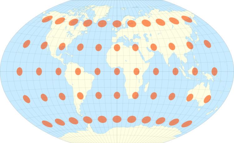
If the region of the map is small enough to ignore Earth's curvature—a town plan, for example—then a single value can be used as the scale without causing measurement errors. In maps covering larger areas, or the whole Earth, the map's scale may be less useful or even useless in measuring distances. The map projection becomes critical in understanding how scale varies throughout the map. When scale varies noticeably, it can be accounted for as the scale factor. Tissot's indicatrix is often used to illustrate the variation of point scale across a map.
Representation of scale
Map scales may be expressed in words (a lexical scale), as a ratio, or as a fraction. Examples are:
Bar scale vs. lexical scale
In addition to the above many maps carry one or more (graphical) bar scales. For example, some modern British maps have three bar scales, one each for kilometres, miles and nautical miles.
A lexical scale on a recently published map, in a language known to the user, may be easier for a non-mathematician to visualise than a ratio: if the scale is an inch to two miles and he can see that two villages are about two inches apart on the map then it is easy to work out that they are about four miles apart on the ground.
A lexical scale may cause problems if it expressed in a language that the user does not understand or in obsolete or ill-defined units. For example, a scale of one inch to a furlong (1:7920) will be understood by many older people in countries where Imperial units used to be taught in schools. But a scale of one pouce to one league may be about 1:144,000 but it depends on the cartographer's choice of the many possible definitions for a league, and only a minority of modern users will be familiar with the units used.
Large scale, medium scale, small scale
Contrast to spatial scale.A map is classified as small scale or large scale or sometimes medium scale. Small scale refers to world maps or maps of large regions such as continents or large nations. In other words, they show large areas of land on a small space. They are called small scale because the representative fraction is relatively small.
Large scale maps show smaller areas in more detail, such as county maps or town plans might. Such maps are called large scale because the representative fraction is relatively large. For instance a town plan, which is a large scale map, might be on a scale of 1:10,000, whereas the world map, which is a small scale map, might be on a scale of 1:100,000,000.
The following table describes typical ranges for these scales but should not be considered authoritative because there is no standard:
The terms are sometimes used in the absolute sense of the table, but other times in a relative sense. For example, a map reader whose work refers solely to large-scale maps (as tabulated above) might refer to a map at 1:500,000 as small-scale.
Scale variation
Mapping large areas causes noticeable distortions due to flattening the significantly curved surface of the earth. How distortion gets distributed depends on the map projection. Scale varies across the map, and the stated map scale will only be an approximation. This is discussed in detail below.
Large-scale maps with curvature neglected
The region over which the earth can be regarded as flat depends on the accuracy of the survey measurements. If measured only to the nearest metre, then curvature of the earth is undetectable over a meridian distance of about 100 kilometres (62 mi) and over an east-west line of about 80 km (at a latitude of 45 degrees). If surveyed to the nearest 1 millimetre (0.039 in), then curvature is undetectable over a meridian distance of about 10 km and over an east-west line of about 8 km. Thus a plan of New York City accurate to one metre or a building site plan accurate to one millimetre would both satisfy the above conditions for the neglect of curvature. They can be treated by plane surveying and mapped by scale drawings in which any two points at the same distance on the drawing are at the same distance on the ground. True ground distances are calculated by measuring the distance on the map and then multiplying by the inverse of the scale fraction or, equivalently, simply using dividers to transfer the separation between the points on the map to a bar scale on the map.
Altitude reduction
The variation in altitude, from the ground level down to the sphere's or ellipsoid's surface, also changes the scale of distance measurements.
Point scale (or particular scale)
As proved by Gauss’s Theorema Egregium, a sphere (or ellipsoid) cannot be projected onto a plane without distortion. This is commonly illustrated by the impossibility of smoothing an orange peel onto a flat surface without tearing and deforming it. The only true representation of a sphere at constant scale is another sphere such as a globe.
Given the limited practical size of globes, we must use maps for detailed mapping. Maps require projections. A projection implies distortion: A constant separation on the map does not correspond to a constant separation on the ground. While a map may display a graphical bar scale, the scale must be used with the understanding that it will be accurate on only some lines of the map. (This is discussed further in the examples in the following sections.)
Let P be a point at latitude
Definition: the point scale at P is the ratio of the two distances P'Q' and PQ in the limit that Q approaches P. We write this as
where the notation indicates that the point scale is a function of the position of P and also the direction of the element PQ.
Definition: if P and Q lie on the same meridian
Definition: if P and Q lie on the same parallel
Definition: if the point scale depends only on position, not on direction, we say that it is isotropic and conventionally denote its value in any direction by the parallel scale factor
Definition: A map projection is said to be conformal if the angle between a pair of lines intersecting at a point P is the same as the angle between the projected lines at the projected point P', for all pairs of lines intersecting at point P. A conformal map has an isotropic scale factor. Conversely isotropic scale factors across the map imply a conformal projection.
Isotropy of scale implies that small elements are stretched equally in all directions, that is the shape of a small element is preserved. This is the property of orthomorphism (from Greek 'right shape'). The qualification 'small' means that at some given accuracy of measurement no change can be detected in the scale factor over the element. Since conformal projections have an isotropic scale factor they have also been called orthomorphic projections. For example, the Mercator projection is conformal since it is constructed to preserve angles and its scale factor is isotopic, a function of latitude only: Mercator does preserve shape in small regions.
Definition: on a conformal projection with an isotropic scale, points which have the same scale value may be joined to form the isoscale lines. These are not plotted on maps for end users but they feature in many of the standard texts. (See Snyder pages 203—206.)
The representative fraction (RF) or principal scale
There are two conventions used in setting down the equations of any given projection. For example, the equirectangular cylindrical projection may be written as
cartographers:Here we shall adopt the first of these conventions (following the usage in the surveys by Snyder). Clearly the above projection equations define positions on a huge cylinder wrapped around the Earth and then unrolled. We say that these coordinates define the projection map which must be distinguished logically from the actual printed (or viewed) maps. If the definition of point scale in the previous section is in terms of the projection map then we can expect the scale factors to be close to unity. For normal tangent cylindrical projections the scale along the equator is k=1 and in general the scale changes as we move off the equator. Analysis of scale on the projection map is an investigation of the change of k away from its true value of unity.
Actual printed maps are produced from the projection map by a constant scaling denoted by a ratio such as 1:100M (for whole world maps) or 1:10000 (for such as town plans). To avoid confusion in the use of the word 'scale' this constant scale fraction is called the representative fraction (RF) of the printed map and it is to be identified with the ratio printed on the map. The actual printed map coordinates for the equirectangular cylindrical projection are
printed map:This convention allows a clear distinction of the intrinsic projection scaling and the reduction scaling.
From this point we ignore the RF and work with the projection map.
Visualisation of point scale: the Tissot indicatrix
Consider a small circle on the surface of the Earth centred at a point P at latitude
Point scale for normal cylindrical projections of the sphere
The key to a quantitative understanding of scale is to consider an infinitesimal element on the sphere. The figure shows a point P at latitude
Normal cylindrical projections of the sphere have
Note that the parallel scale factor
The following examples illustrate three normal cylindrical projections and in each case the variation of scale with position and direction is illustrated by the use of Tissot's indicatrix.
The equirectangular projection
The equirectangular projection, also known as the Plate Carrée (French for "flat square") or (somewhat misleadingly) the equidistant projection, is defined by
where
Since
For the calculation of the point scale in an arbitrary direction see addendum.
The figure illustrates the Tissot indicatrix for this projection. On the equator h=k=1 and the circular elements are undistorted on projection. At higher latitudes the circles are distorted into an ellipse given by stretching in the parallel direction only: there is no distortion in the meridian direction. The ratio of the major axis to the minor axis is
It is instructive to consider the use of bar scales that might appear on a printed version of this projection. The scale is true (k=1) on the equator so that multiplying its length on a printed map by the inverse of the RF (or principal scale) gives the actual circumference of the Earth. The bar scale on the map is also drawn at the true scale so that transferring a separation between two points on the equator to the bar scale will give the correct distance between those points. The same is true on the meridians. On a parallel other than the equator the scale is
Mercator projection
The Mercator projection maps the sphere to a rectangle (of infinite extent in the
where a,
In the mathematical addendum it is shown that the point scale in an arbitrary direction is also equal to
Lambert's equal area projection
Lambert's equal area projection maps the sphere to a finite rectangle by the equations
where a,
The calculation of the point scale in an arbitrary direction is given below.
The vertical and horizontal scales now compensate each other (hk=1) and in the Tissot diagram each infinitesimal circular element is distorted into an ellipse of the same area as the undistorted circles on the equator.
Graphs of scale factors
The graph shows the variation of the scale factors for the above three examples. The top plot shows the isotropic Mercator scale function: the scale on the parallel is the same as the scale on the meridian. The other plots show the meridian scale factor for the Equirectangular projection (h=1) and for the Lambert equal area projection. These last two projections have a parallel scale identical to that of the Mercator plot. For the Lambert note that the parallel scale (as Mercator A) increases with latitude and the meridian scale (C) decreases with latitude in such a way that hk=1, guaranteeing area conservation.
Scale variation on the Mercator projection
The Mercator point scale is unity on the equator because it is such that the auxiliary cylinder used in its construction is tangential to the Earth at the equator. For this reason the usual projection should be called a tangent projection. The scale varies with latitude as
A standard criterion for good large-scale maps is that the accuracy should be within 4 parts in 10,000, or 0.04%, corresponding to
Secant, or modified, projections
The basic idea of a secant projection is that the sphere is projected to a cylinder which intersects the sphere at two parallels, say
As an example, one possible secant Mercator projection is defined by
The numeric multipliers do not alter the shape of the projection but it does mean that the scale factors are modified:
Thus
This is illustrated by the lower (green) curve in the figure of the previous section.
Such narrow zones of high accuracy are used in the UTM and the British OSGB projection, both of which are secant, transverse Mercator on the ellipsoid with the scale on the central meridian constant at
The lines of unit scale at latitude
Whilst a narrow band with
The scale plots for the latter are shown below compared with the Lambert equal area scale factors. In the latter the equator is a single standard parallel and the parallel scale increases from k=1 to compensate the decrease in the meridian scale. For the Gall the parallel scale is reduced at the equator (to k=0.707) whilst the meridian scale is increased (to k=1.414). This gives rise to the gross distortion of shape in the Gall-Peters projection. (On the globe Africa is about as long as it is broad). Note that the meridian and parallel scales are both unity on the standard parallels.
Mathematical addendum
For normal cylindrical projections the geometry of the infinitesimal elements gives
The relationship between the angles
For the Mercator projection
Setting
For the projections other than Mercator we must first calculate
If we consider a line of constant slope