
 | ||
Similar Paris meridian, Seconds pendulum, Struve Geodetic Arc | ||
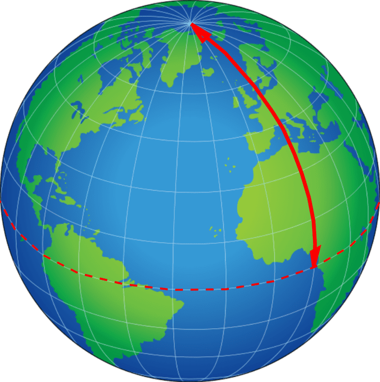
In geodesy, a meridian arc measurement is the distance between two points with the same longitude, i.e., a segment of a meridian curve or its length. Two or more such determinations at different locations then specify the shape of the reference ellipsoid which best approximates the shape of the geoid. This process is called the determination of the Figure of the Earth. The earliest determinations of the size of a spherical Earth required a single arc. The latest determinations use astro-geodetic measurements and the methods of satellite geodesy to determine the reference ellipsoids.
Contents
- The Earth as a sphere
- The Earth as an ellipsoid
- The seventeenth and eighteenth centuries
- The nineteenth century
- Meridian distance on the ellipsoid
- Relation to elliptic integrals
- Series expansions
- Expansions in the eccentricity e
- Expansions in the third flattening n
- Series in terms of the parametric latitude
- Generalized series
- Numerical expressions
- The inverse meridian problem for the ellipsoid
- References
Those interested in accurate expressions of the meridian arc for the WGS84 ellipsoid should consult the subsection entitled numerical expressions.
The Earth as a sphere
Early estimations of Earth's size are recorded from Greece in the 4th century BC, and from scholars at the caliph's House of Wisdom in the 9th century. The first realistic value was calculated by Alexandrian scientist Eratosthenes about 240 BC. He knew that on the summer solstice at local noon the sun goes through the zenith in the ancient Egyptian city of Syene (Assuan). He also knew from his own measurements that, at the same moment in his hometown of Alexandria, the zenith distance was 1/50 of a full circle (7.2°).
Assuming that Alexandria was due north of Syene, Eratosthenes concluded that the distance between Alexandria and Syene must be 1/50 of Earth's circumference. Using data from caravan travels, he estimated the distance to be 5,000 stadia (about 500 nautical miles)—which implies a circumference of 252,000 stadia. Assuming the Attic stadion (185 m) this corresponds to 46,620 km, or 16% too great. However, if Eratosthenes used the Egyptian stadion (157.5 m) his measurement turns out to be 39,690 km, an error of only 1%. Syene is not precisely on the Tropic of Cancer and not directly south of Alexandria. The sun appears as a disk of 0.5°, and an estimate of the overland distance traveling along the Nile or through the desert couldn't be more accurate than about 10%.
Eratosthenes' estimation of Earth's size was accepted for nearly two thousand years. A similar method was used by Posidonius about 150 years later, and slightly better results were calculated in 827 by the grade measurement of the Caliph Al-Ma'mun.
The Earth as an ellipsoid
Early literature uses the term oblate spheroid to describe a sphere "squashed at the poles". Modern literature uses the term "ellipsoid of revolution" in place of spheroid, although the qualifying words "of revolution" are usually dropped. An ellipsoid which is not an ellipsoid of revolution is called a triaxial ellipsoid. Spheroid and ellipsoid are used interchangeably in this article, with oblate implied if not stated.
The seventeenth and eighteenth centuries
In 1687 Newton had published in the Principia a proof that the earth was an oblate spheroid of flattening equal to 1/230. This was disputed by some, but not all, French scientists. A meridian arc of Jean Picard was extended to a longer arc by Giovanni Domenico Cassini and his son Jacques Cassini over the period 1684–1718. The arc was measured with at least three latitude determinations, so they were able to deduce mean curvatures for the northern and southern halves of the arc, allowing a determination of the overall shape. The results indicated that the Earth was a prolate spheroid (with an equatorial radius less than the polar radius). To resolve the issue, the French Academy of Sciences (1735) proposed expeditions to Peru (Bouguer, Louis Godin, de La Condamine, Antonio de Ulloa, Jorge Juan) and Lapland (Maupertuis, Clairaut, Camus, Le Monnier, Abbe Outhier, Celsius). The expedition to Peru is described in the French Geodesic Mission article and that to Lapland is described in the Torne Valley article. The resulting measurements at equatorial and polar latitudes confirmed that the earth was best modelled by an oblate spheroid, supporting Newton.
By the end of the century Delambre had remeasured and extended the French arc from Dunkirk to the Mediterranean. It was divided into five parts by four intermediate determinations of latitude. By combining the measurements together with those for the arc of Peru, ellipsoid shape parameters were determined and the distance between the equator and pole along the Paris Meridian was calculated as 7006513076200000000♠5130762 toises as specified by the standard toise bar in Paris. Defining this distance as exactly 7007100000000000000♠10000000 m led to the construction of a new standard metre bar as 6999513076200000000♠0.5130762 toises.
The nineteenth century
In the 19th century, many astronomers and geodesists were engaged in detailed studies of the Earth's curvature along different meridian arcs. The analyses resulted in a great many model ellipsoids such as Plessis 1817, Airy 1830, Bessel 1830, Everest 1830, and Clarke 1866. A comprehensive list of ellipsoids is given under Earth ellipsoid.
Meridian distance on the ellipsoid
The determination of the meridian distance, that is the distance from the equator to a point at a latitude φ on the ellipsoid is an important problem in the theory of map projections, particularly the Transverse Mercator projection. Ellipsoids are normally specified in terms of the parameters defined above, a, b, f, but in theoretical work it is useful to define extra parameters, particularly the eccentricity, e, and the third flattening n. Only two of these parameters are independent and there are many relations between them:
The meridian radius of curvature can be shown to be equal to
so that the arc length of an infinitesimal element of the meridian is dm = M(φ) dφ (with φ in radians). Therefore, the meridian distance from the equator to latitude φ is
The distance formula is simpler when written in terms of the parametric latitude,
where tan β = (1 − f)tan φ and e′2 = e2/1 − e2.
The distance from the equator to the pole, the quarter meridian, is
Even though latitude is normally confined to the range [−π/2,π/2], all the formulae given here apply to measuring distance around the complete meridian ellipse (including the anti-meridian). Thus the ranges of φ, β, and the rectifying latitude μ, are unrestricted.
Relation to elliptic integrals
The above integral is related to a special case of an incomplete elliptic integral of the third kind. In the notation of the online NIST handbook (Section 19.2(ii)),
It may also be written in terms of incomplete elliptic integrals of the second kind (See the NIST handbook Section 19.6(iv)),
The quarter meridian can be expressed in terms of the complete elliptic integral of the second kind,
The calculation (to arbitrary precision) of the elliptic integrals and approximations are also discussed in the NIST handbook. These functions are also implemented in computer algebra programs such as Mathematica and Maxima.
Series expansions
The above integral may be expressed as an infinite truncated series by expanding the integrand in a Taylor series, performing the resulting integrals term by term, and expressing the result as a trigonometric series. In 1755, Euler derived an expansion in the third eccentricity squared.
Expansions in the eccentricity (e)
Delambre in 1799 derived a widely used expansion on e2,
where
Rapp gives a detailed derivation of this result. In this article, trigonometric terms of the form sin 4φ are interpreted as sin(4φ).
Expansions in the third flattening (n)
Series with considerably faster convergence can be obtained by expanding in terms of the third flattening n instead of the eccentricity. They are related by
In 1837, Bessel obtained one such series, which was put into a simpler form by Helmert,
with
Because n changes sign when a and b are interchanged, and because the initial factor 1/2(a + b) is constant under this interchange, half the terms in the expansions of H2k vanish.
The series can be expressed with either a or b as the initial factor by writing, for example,
and expanding the result as a series in n. Even though this results in more slowly converging series, such series are used in the specification for the transverse Mercator projection by the National Geospatial Intelligence Agency and the Ordnance Survey of Great Britain.
Series in terms of the parametric latitude
In 1825, Bessel derived an expansion of the meridian distance in terms of the parametric latitude β in connection with his work on geodesics,
with
Because this series provides an expansion for the elliptic integral of the second kind, it can be used to write the arc length in terms of the geographic latitude as
Generalized series
The above series, to eighth order in eccentricity or fourth order in third flattening, provide millimetre accuracy. With the aid of symbolic algebra systems, they can easily be extended to sixth order in the third flattening which provides full double precision accuracy for terrestrial applications.
Delambre and Bessel both wrote their series in a form that allows them to be generalized to arbitrary order. The coefficients in Bessel's series can expressed particularly simply
where
and k!! is the double factorial, extended to negative values via the recursion relation: (−1)!! = 1 and (−3)!! = −1.
The coefficients in Helmert's series can similarly be expressed generally by
This result was conjected by Helmert and proved by Kawase.
The factor (1 − 2k)(1 + 2k) results in poorer convergence of the series in terms of φ compared to the one in β.
The quarter meridian is given by
a result which was first obtained by Ivory.
Numerical expressions
The trigonometric series given above can be conveniently evaluated using Clenshaw summation. This method avoids the calculation of most of the trigonometric functions and allows the series to be summed rapidly and accurately. The technique can also be used to evaluate the difference m(φ1) − m(φ2) while maintaining high relative accuracy.
Substituting the values for the semi-major axis and eccentricity of the WGS84 ellipsoid gives
where φ(°) = φ/1° is φ expressed in degrees (and similarly for β(°)).
For the WGS84 ellipsoid the quarter meridian is
The perimeter of a meridian ellipse is 4mp = 2π(a + b)c0. Therefore, 1/2(a + b)c0 is the radius of the circle whose circumference is the same as the perimeter of a meridian ellipse. This defines the rectifying Earth radius as 7006636744914600000♠6367449.146 m.
On the ellipsoid the exact distance between parallels at φ1 and φ2 is m(φ1) − m(φ2). For WGS84 an approximate expression for the distance Δm between the two parallels at 0.5° from the circle at latitude φ is given by
The inverse meridian problem for the ellipsoid
In some problems, we need to be able to solve the inverse problem: given m, determine φ. This may be solved by Newton's method, iterating
until convergence. A suitable starting guess is given by φ0 = μ where
is the rectifying latitude. Note that it there is no need to differentiate the series for m(φ), since the formula for the meridian radius of curvature M(φ) can be used instead.
Alternatively, Helmert's series for the meridian distance can be reverted to give
where
Similarly, Bessel's series for m in terms of β can be reverted to give
where
Legendre showed that the distance along a geodesic on an spheroid is the same as the distance along the perimeter of an ellipse. For this reason, the expression for m in terms of β and its inverse given above play a key role in the solution of the geodesic problem with m replaced by s, the distance along the geodesic, and β replaced by σ, the arc length on the auxiliary sphere. The requisite series extended to sixth order are given by Karney, Eqs. (17) & (21), with ε playing the role of n and τ playing the role of μ.