Sample complexity

Definition

Let X be a space which we call the input space, and Y be a space which we call the output space, and let Z denote the product X × Y . For example, in the setting of binary classification, X is typically a finite-dimensional vector space and Y is the set { − 1 , 1 } .

Fix a hypothesis space H of functions h : X → Y . A learning algorithm over H is a computable map from Z ∗ to H . In other words, it is an algorithm that takes as input a finite sequence of training samples and outputs a function from X to Y . Typical learning algorithms include empirical risk minimization, without or with Tikhonov regularization.

Fix a loss function L o s s : Y × Y → R ≥ 0 , for example, the square loss L o s s ( y , y ′ ) = ( y − y ′ ) 2 . For a given distribution ρ on X × Y , the expected risk of a hypothesis (a function) h ∈ H is

In our setting, we have h = A L G ( S n ) where A L G is a learning algorithm and S n = ( ( x 1 , y 1 ) , … , ( x n , y n ) ) ∼ ρ n is a sequence of vectors which are all drawn independently from ρ . Define the optimal risk

In words, the sample complexity N ( ρ , ϵ , δ ) defines the rate of consistency of the algorithm: given a desired accuracy ε and confidence δ, one needs to sample N ( ρ , ϵ , δ ) data points to guarantee that the risk of the output function is within ε of the best possible, with probability at least 1 - δ.

In probabilistically approximately correct (PAC) learning, one is concerned with whether the sample complexity is polynomial, that is, whether N ( ρ , ϵ , δ ) is bounded by a polynomial in 1/ε and 1/δ. If N ( ρ , ϵ , δ ) is polynomial for some learning algorithm, then one says that the hypothesis space H is PAC-learnable. Note that this is a stronger notion than being learnable.

Unrestricted hypothesis space: infinite sample complexity

One can ask whether there exists a learning algorithm so that the sample complexity is finite in the strong sense, that is, there is a bound on the number of samples needed so that the algorithm can learn any distribution over the input-output space with a specified target error. More formally, one asks whether there exists a learning algorithm A L G such that, for all ε, δ > 0, there exists a positive integer N such that for all n ≥ N, we have

Thus, in order to make statements about the rate of convergence of the quantity

Restricted hypothesis space: finite sample-complexity

The latter approach leads to concepts such as VC dimension and Rademacher complexity which control the complexity of the space H . A smaller hypothesis space introduces more bias into the inference process, meaning that E H ∗ may be greater than the best possible risk in a larger space. However, by restricting the complexity of the hypothesis space it becomes possible for an algorithm to produce more uniformly consistent functions. This trade-off leads to the concept of regularization.

It is a theorem from VC theory that the following three statements are equivalent for a hypothesis space H :

1. H is PAC-learnable.
2. The VC dimension of H is finite.
3. H is a uniform Glivenko-Cantelli class.

This gives a way to prove that certain hypothesis spaces are PAC learnable, and by extension, learnable.

An example of a PAC-learnable hypothesis space

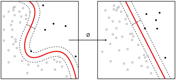
Let X = R^d, Y = {-1, 1}, and let H be the space of affine functions on X, that is, functions of the form x ↦ ⟨ w , x ⟩ + b for some w ∈ R d , b ∈ R . This is the linear classification with offset learning problem. Now, note that four coplanar points in a square cannot be shattered by any affine function, since no affine function can be positive on two diagonally opposite vertices and negative on the remaining two. Thus, the VC dimension of H is 3, in particular finite. It follows by the above characterization of PAC-learnable classes that H is PAC-learnable, and by extension, learnable.

Sample-complexity bounds

Suppose H is a class of binary functions (functions to {0,1}). Then, H is ( ϵ , δ ) -PAC-learnable with a sample of size:

Suppose H is a class of real-valued functions with range in [0,T]. Then, H is ( ϵ , δ ) -PAC-learnable with a sample of size:

Other Settings

In addition to the supervised learning setting, sample complexity is relevant to semi-supervised learning problems including active learning, where the algorithm can ask for labels to specifically chosen inputs in order to reduce the cost of obtaining many labels. The concept of sample complexity also shows up in reinforcement learning, online learning, and unsupervised algorithms, e.g. for dictionary learning.