
 | ||
First developed in 1985 by RockWare Inc, RockWorks is used by the mining, petroleum, and environmental industry for subsurface visualization, borehole database management as well as the creation of grids, solid models, calculating volumetric analysis, etc.
Contents
RockWorks background
Computer modeling in RockWorks provides a means for tailoring a mine, environmental, petroleum, etc. plan based on the end-user specifications. The basic strategy involves the creation of a borehole database that includes analytical results for various physical and chemical properties as a function of depth. Once the database has been created, visualizations such as cross-sections, fence diagrams, and block diagrams are generated to check the validity and geological reasonability of the modeling. The next steps can involve the calculation of volumetrics and optimal pit-designs for example, in mining, based on a series of user-defined parameters.
The foundation of these analyses involve the creation of imaginary block models in which a site is subdivided into a series of three-dimensional cells called a voxel (volumetric element). Values are estimated for these voxels based on their proximity relative to downhole data. For example, a clay deposit may involve the creation of separate models representing shrinkage, brightness, and slip. These models are then filtered and combined into a final model that shows where all of the parameters (models) meet a set of user-defined criteria. The net result is high-grade, or “surgical” mining in which the quarry is designed to maximize profitability rather than simply mining the entire lease and relying on the sorting/milling process to separate the ore and the non-ore.
A healthy level of skepticism must be employed when using computer software to compute resource volumetrics. The algorithms or methods used to create the volumetric models have limitations that may be acceptable for one type of deposit while being completely inappropriate for another. For example, a sand and gravel deposit requires an approach that is completely different from the methods used to evaluate a phosphate reserve. The best way to avoid misuse is to always compare “slices” through the models with borehole logs that show the original data. These cross-sections are used to make sure that the model “honors” the data. Just as importantly, cross-sections should be evaluated to make sure that the modeling conforms to the expected geology.
The raw dataset that are used for industrial mineral deposit modeling can be classified into two major types: borehole and non-borehole data. The management of borehole data is very different from non-borehole data. Specifically, borehole data requires a relational database management system (e.g. Access, FileMaker, SQL, Oracle,) whereas non-borehole data (with the exception of land ownership) can be handled with simple “flat” file managers (e.g. Microsoft Excel, Lotus 1-2-3).
Modeling
“Modeling” refers to the process of creating a spatial array of estimations. The parameter that is being estimated may be the thickness of the ore, the grade of the ore, or some other property that is useful for the evaluation of the resource. These arrays may be two or three-dimensional depending upon the number of independent variables. In a two-dimensional array (also referred to as a “grid model”), the dependent variable (z) is a function of the horizontal (x,y) coordinates. In a three-dimensional array (also referred to as a solid or block model), the dependent variable (g) is a function of the horizontal (x,y) and vertical coordinates (z). Grids are used to model topography, stratigraphic contacts, isopachs, and water levels, while solids are used to model geochemistry, ore grades, and geotechnical properties.
The key difference between grid models and block models is that a gridded surface (e.g. a stratigraphic contact) cannot fold or wrap under itself whereas an isosurface within a block model can. Stated differently, when dealing with grids, there can only be one z-value for any given xy coordinate. On the other hand, when dealing with block models, there can only be one g-value for any given xyz coordinate. Another major difference is that gridding is computationally fast while block modeling can be very slow.
Two-Dimensional Modeling (Gridding)
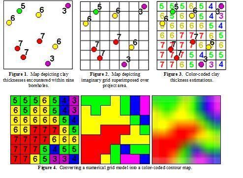
Consider the evaluation of a clay deposit in which the only important parameter is the thickness of the clay (i.e. the clay grade is homogeneous or “anisotropic”). Variations in the clay thickness encountered within nine boreholes are depicted by Figure 1.
The first step in the modeling process is to superimpose an imaginary grid (Figure 2) over the project area. This grid defines the resolution of the subsequent model in a manner analogous to pixels (picture elements) within a digital image. Specifically, as the pixels become smaller, smaller features are resolved at the expense of computer memory and speed. A general guideline for dimensioning the grid is to set the cell dimensions equal to the average minimum distance between the control points (e.g. boreholes).
Once a grid has been established, the clay thicknesses at the center of each grid node are estimated. These estimations are based on a weighted average of the values associated with the surrounding control points (Figure 3). A variety of interpolation methods or “algorithms” are available for performing these estimations. A popular and simple technique called inverse distance weighting (IDW) varies the influence of surrounding points based on the inverse of the distance between the control point and the interpolated point. Another technique, called Kriging varies the influence of surrounding points based on a statistical analysis of their relative distance and direction.
Grid models are commonly used to produce color-coded contour maps by averaging the regions between cells (Figure 4). In fact, most computer contouring uses gridding as a preliminary, behind-the-scenes, step towards producing contours. There are, however, many more things that can be done with grids, including volumetrics.
Three-Dimensional Block Modeling
Block modeling (Figure 1) is simply the three-dimensional version of gridding. The original data points typically consist of quantitative downhole data (e.g. geochemistry, ore grades, physical properties, etc.).
Software Versions
RockWare will discontinue their technical support and unlocking for any version prior to RockWorks15 after 12/31/2015.
RockWorks is currently on version 17 which was released on October 19, 2015. As of November 10, 2016, there have been 752 updates to the software since its development RockWorks17 is the first 64bit version of the software. This new version also moves away from an MS Access database format to a native SQLite database format as well as the capability to utilize other database engines and Enterprise Database products.
The software is designed to analyze and visualize interval and point data such as stratigraphy, lithology, quantitative data, color intervals, fracture data and hydrology and aquifer data. The software is extensively used in the Geotechnical, Environmental, Mining, and Petroleum industries.
Some of the functions of the software include:
The software comes in 3 Levels of capability after download for a limited time, but even after the trial period is over it still serves as a reader of all the file types and has the Earth Apps capability which allows output of files to Google Earth via creation of .klm files. Licensing of the software can be standalone computer license or network licensing. Software purchased from the company comes with a 30 minutes of phone support and email support from actual in-house geologists (not outsourced tech support) as long as your software is the current or previous version.
Revision History
For information about specific current version fixes: https://www.rockware.com/rockworks/revisions/current_revisions.htm