
 | ||
A restricted Boltzmann machine (RBM) is a generative stochastic artificial neural network that can learn a probability distribution over its set of inputs.
Contents
RBMs were initially invented under the name Harmonium by Paul Smolensky in 1986, and rose to prominence after Geoffrey Hinton and collaborators invented fast learning algorithms for them in the mid-2000s. RBMs have found applications in dimensionality reduction, classification, collaborative filtering, feature learning and topic modelling. They can be trained in either supervised or unsupervised ways, depending on the task.
As their name implies, RBMs are a variant of Boltzmann machines, with the restriction that their neurons must form a bipartite graph: a pair of nodes from each of the two groups of units (commonly referred to as the "visible" and "hidden" units respectively) may have a symmetric connection between them; and there are no connections between nodes within a group. By contrast, "unrestricted" Boltzmann machines may have connections between hidden units. This restriction allows for more efficient training algorithms than are available for the general class of Boltzmann machines, in particular the gradient-based contrastive divergence algorithm.
Restricted Boltzmann machines can also be used in deep learning networks. In particular, deep belief networks can be formed by "stacking" RBMs and optionally fine-tuning the resulting deep network with gradient descent and backpropagation.
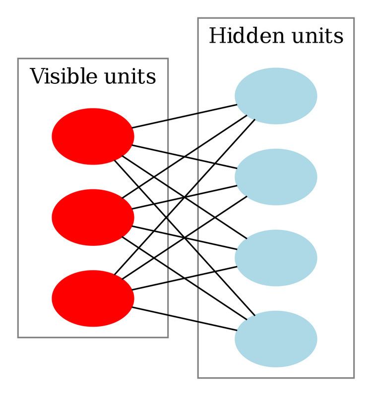
Structure
The standard type of RBM has binary-valued (Boolean/Bernoulli) hidden and visible units, and consists of a matrix of weights
or, in matrix notation,
This energy function is analogous to that of a Hopfield network. As in general Boltzmann machines, probability distributions over hidden and/or visible vectors are defined in terms of the energy function:
where
Since the RBM has the shape of a bipartite graph, with no intra-layer connections, the hidden unit activations are mutually independent given the visible unit activations and conversely, the visible unit activations are mutually independent given the hidden unit activations. That is, for
Conversely, the conditional probability of h given v is
The individual activation probabilities are given by
where
The visible units of RBM can be multinomial, although the hidden units are Bernoulli. In this case, the logistic function for visible units is replaced by the softmax function
where K is the number of discrete values that the visible values have. They are applied in topic modeling, and recommender systems.
Relation to other models
Restricted Boltzmann machines are a special case of Boltzmann machines and Markov random fields. Their graphical model corresponds to that of factor analysis.
Training algorithm
Restricted Boltzmann machines are trained to maximize the product of probabilities assigned to some training set
or equivalently, to maximize the expected log probability of a training sample
The algorithm most often used to train RBMs, that is, to optimize the weight vector
The basic, single-step contrastive divergence (CD-1) procedure for a single sample can be summarized as follows:
- Take a training sample v, compute the probabilities of the hidden units and sample a hidden activation vector h from this probability distribution.
- Compute the outer product of v and h and call this the positive gradient.
- From h, sample a reconstruction v' of the visible units, then resample the hidden activations h' from this. (Gibbs sampling step)
- Compute the outer product of v' and h' and call this the negative gradient.
- Let the update to the weight matrix
W be the positive gradient minus the negative gradient, times some learning rate:Δ W = ϵ ( v h T − v ′ h ′ T ) . - Update the biases a and b analogously:
Δ a = ϵ ( v − v ′ ) ,Δ b = ϵ ( h − h ′ ) .
A Practical Guide to Training RBMs written by Hinton can be found on his homepage.