Recurrent neural network

Fully recurrent network

This is the basic architecture developed in the 1980s: a network of neuron-like units, each with a directed connection to every other unit. Each unit has a time-varying real-valued activation. Each connection has a modifiable real-valued weight. Some of the nodes are called input nodes, some output nodes, the rest hidden nodes. Most architectures below are special cases.

For supervised learning in discrete time settings, training sequences of real-valued input vectors become sequences of activations of the input nodes, one input vector at a time. At any given time step, each non-input unit computes its current activation as a nonlinear function of the weighted sum of the activations of all units from which it receives connections. There may be teacher-given target activations for some of the output units at certain time steps. For example, if the input sequence is a speech signal corresponding to a spoken digit, the final target output at the end of the sequence may be a label classifying the digit. For each sequence, its error is the sum of the deviations of all target signals from the corresponding activations computed by the network. For a training set of numerous sequences, the total error is the sum of the errors of all individual sequences. Algorithms for minimizing this error are mentioned in the section on training algorithms below.

In reinforcement learning settings, there is no teacher providing target signals for the RNN, instead a fitness function or reward function is occasionally used to evaluate the RNN's performance, which is influencing its input stream through output units connected to actuators affecting the environment. Again, compare the section on training algorithms below.

Recursive neural networks

A recursive neural network is created by applying the same set of weights recursively over a differentiable graph-like structure, by traversing the structure in topological order. Such networks are typically also trained by the reverse mode of automatic differentiation. They were introduced to learn distributed representations of structure, such as logical terms. A special case of recursive neural networks is the RNN itself whose structure corresponds to a linear chain. Recursive neural networks have been applied to natural language processing. The Recursive Neural Tensor Network uses a tensor-based composition function for all nodes in the tree.

Hopfield network

The Hopfield network is of historic interest although it is not a general RNN, as it is not designed to process sequences of patterns. Instead it requires stationary inputs. It is a RNN in which all connections are symmetric. Invented by John Hopfield in 1982, it guarantees that its dynamics will converge. If the connections are trained using Hebbian learning then the Hopfield network can perform as robust content-addressable memory, resistant to connection alteration.

A variation on the Hopfield network is the bidirectional associative memory (BAM). The BAM has two layers, either of which can be driven as an input, to recall an association and produce an output on the other layer.

Elman networks and Jordan networks

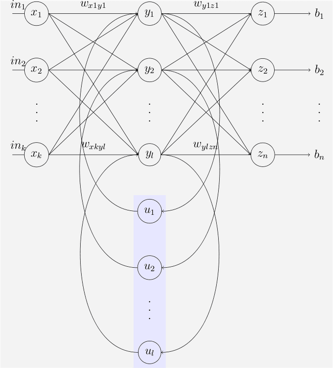
The following special case of the basic architecture above was employed by Jeff Elman. A three-layer network is used (arranged horizontally as x, y, and z in the illustration), with the addition of a set of "context units" (u in the illustration). There are connections from the middle (hidden) layer to these context units fixed with a weight of one. At each time step, the input is propagated in a standard feed-forward fashion, and then a learning rule is applied. The fixed back connections result in the context units always maintaining a copy of the previous values of the hidden units (since they propagate over the connections before the learning rule is applied). Thus the network can maintain a sort of state, allowing it to perform such tasks as sequence-prediction that are beyond the power of a standard multilayer perceptron.

Jordan networks, due to Michael I. Jordan, are similar to Elman networks. The context units are however fed from the output layer instead of the hidden layer. The context units in a Jordan network are also referred to as the state layer, and have a recurrent connection to themselves with no other nodes on this connection.

Elman and Jordan networks are also known as "simple recurrent networks" (SRN).

Variables and functions

Echo state network

The echo state network (ESN) is a recurrent neural network with a sparsely connected random hidden layer. The weights of output neurons are the only part of the network that can change and be trained. ESN are good at reproducing certain time series. A variant for spiking neurons is known as liquid state machines.

Neural history compressor

The vanishing gradient problem of automatic differentiation or backpropagation in neural networks was partially overcome in 1992 by an early generative model called the neural history compressor, implemented as an unsupervised stack of recurrent neural networks (RNNs). The RNN at the input level learns to predict its next input from the previous input history. Only unpredictable inputs of some RNN in the hierarchy become inputs to the next higher level RNN which therefore recomputes its internal state only rarely. Each higher level RNN thus learns a compressed representation of the information in the RNN below. This is done such that the input sequence can be precisely reconstructed from the sequence representation at the highest level. The system effectively minimises the description length or the negative logarithm of the probability of the data. If there is a lot of learnable predictability in the incoming data sequence, then the highest level RNN can use supervised learning to easily classify even deep sequences with very long time intervals between important events. In 1993, such a system already solved a "Very Deep Learning" task that requires more than 1000 subsequent layers in an RNN unfolded in time.

It is also possible to distill the entire RNN hierarchy into only two RNNs called the "conscious" chunker (higher level) and the "subconscious" automatizer (lower level). Once the chunker has learned to predict and compress inputs that are still unpredictable by the automatizer, then the automatizer can be forced in the next learning phase to predict or imitate through special additional units the hidden units of the more slowly changing chunker. This makes it easy for the automatizer to learn appropriate, rarely changing memories across very long time intervals. This in turn helps the automatizer to make many of its once unpredictable inputs predictable, such that the chunker can focus on the remaining still unpredictable events, to compress the data even further.

Long short-term memory

Numerous researchers now use a deep learning RNN called the long short-term memory (LSTM) network, published by Hochreiter & Schmidhuber in 1997. It is a deep learning system that unlike traditional RNNs doesn't have the vanishing gradient problem (compare the section on training algorithms below). LSTM is normally augmented by recurrent gates called forget gates. LSTM RNNs prevent backpropagated errors from vanishing or exploding. Instead errors can flow backwards through unlimited numbers of virtual layers in LSTM RNNs unfolded in space. That is, LSTM can learn "Very Deep Learning" tasks that require memories of events that happened thousands or even millions of discrete time steps ago. Problem-specific LSTM-like topologies can be evolved. LSTM works even when there are long delays, and it can handle signals that have a mix of low and high frequency components.

Today, many applications use stacks of LSTM RNNs and train them by Connectionist Temporal Classification (CTC) to find an RNN weight matrix that maximizes the probability of the label sequences in a training set, given the corresponding input sequences. CTC achieves both alignment and recognition. Around 2007, LSTM started to revolutionise speech recognition, outperforming traditional models in certain speech applications. In 2009, CTC-trained LSTM was the first RNN to win pattern recognition contests, when it won several competitions in connected handwriting recognition. In 2014, the Chinese search giant Baidu used CTC-trained RNNs to break the Switchboard Hub5'00 speech recognition benchmark, without using any traditional speech processing methods. LSTM also improved large-vocabulary speech recognition, text-to-speech synthesis, also for Google Android, and photo-real talking heads. In 2015, Google's speech recognition reportedly experienced a dramatic performance jump of 49% through CTC-trained LSTM, which is now available through Google voice search to all smartphone users.

LSTM has also become very popular in the field of natural language processing. Unlike previous models based on HMMs and similar concepts, LSTM can learn to recognise context-sensitive languages. LSTM improved machine translation, Language Modeling and Multilingual Language Processing. LSTM combined with convolutional neural networks (CNNs) also improved automatic image captioning and a plethora of other applications.

Gated recurrent unit

Gated recurrent unit is one of the recurrent neural network introduced in 2014.

Bi-directional RNN

Invented by Schuster & Paliwal in 1997, bi-directional RNN or BRNN use a finite sequence to predict or label each element of the sequence based on both the past and the future context of the element. This is done by concatenating the outputs of two RNN, one processing the sequence from left to right, the other one from right to left. The combined outputs are the predictions of the teacher-given target signals. This technique proved to be especially useful when combined with LSTM RNN.

Continuous-time RNN

A continuous time recurrent neural network (CTRNN) is a dynamical systems model of biological neural networks. A CTRNN uses a system of ordinary differential equations to model the effects on a neuron of the incoming spike train.

For a neuron i in the network with action potential y i the rate of change of activation is given by:

Where:

CTRNNs have frequently been applied in the field of evolutionary robotics, where they have been used to address, for example, vision, co-operation and minimally cognitive behaviour.

Note that by the Shannon sampling theorem, discrete time recurrent neural networks can be viewed as continuous time recurrent neural networks where the differential equation have transformed in an equivalent difference equation after that the postsynaptic node activation functions y i ( t ) have been low-pass filtered prior to sampling.

Hierarchical RNN

There are many instances of hierarchical RNN whose elements are connected in various ways to decompose hierarchical behavior into useful subprograms.

Recurrent multilayer perceptron

Generally, a Recurrent Multi-Layer Perceptron (RMLP) consists of a series of cascaded subnetworks, each of which consists of multiple layers of nodes. Each of these subnetworks is entirely feed-forward except for the last layer, which can have feedback connections among itself. Each of these subnets is connected only by feed forward connections.

Second order RNN

Second order RNNs use higher order weights w i j k instead of the standard w i j weights, and inputs and states can be a product. This allows a direct mapping to a finite state machine both in training, stability, and representation. Long short-term memory is an example of this but has no such formal mappings or proof of stability.

Multiple timescales recurrent neural network (MTRNN) model

MTRNN is a possible neural-based computational model that imitates to some extent the activity of the brain. It has the ability to simulate the functional hierarchy of the brain through self-organization that not only depends on spatial connection between neurons, but also on distinct types of neuron activities, each with distinct time properties. With such varied neuronal activities, continuous sequences of any set of behaviors are segmented into reusable primitives, which in turn are flexibly integrated into diverse sequential behaviors. The biological approval of such a type of hierarchy has been discussed on the memory-prediction theory of brain function by Jeff Hawkins in his book On Intelligence.

Neural Turing machines

Neural Turing machines (NTMs) are a method of extending the capabilities of recurrent neural networks by coupling them to external memory resources, which they can interact with by attentional processes. The combined system is analogous to a Turing machine or Von Neumann architecture but is differentiable end-to-end, allowing it to be efficiently trained with gradient descent.

Neural network pushdown automata

NNPDAs are similar to NTMs but tapes are replaced by analogue stacks that are differentiable and which are trained to control. In this way they are similar in complexity to recognizers of context free grammars (CFGs).

Bidirectional associative memory

First introduced by Kosko, BAM neural networks store associative data as a vector. The bi-directionality comes from passing information through a matrix and its transpose. Typically, bipolar encoding is preferred to binary encoding of the associative pairs. Recently, stochastic BAM models using Markov stepping were optimized for increased network stability and relevance to real-world applications.

Gradient descent

To minimize total error, gradient descent can be used to change each weight in proportion to the derivative of the error with respect to that weight, provided the non-linear activation functions are differentiable. Various methods for doing so were developed in the 1980s and early 1990s by Paul Werbos, Ronald J. Williams, Tony Robinson, Jürgen Schmidhuber, Sepp Hochreiter, Barak Pearlmutter, and others.

The standard method is called "backpropagation through time" or BPTT, and is a generalization of back-propagation for feed-forward networks, and like that method, is an instance of automatic differentiation in the reverse accumulation mode or Pontryagin's minimum principle. A more computationally expensive online variant is called "Real-Time Recurrent Learning" or RTRL, which is an instance of Automatic differentiation in the forward accumulation mode with stacked tangent vectors. Unlike BPTT this algorithm is local in time but not local in space.

In this context, local in space means that a unit's weight vector can be updated only using information stored in the connected units and the unit itself such that update complexity of a single unit is linear in the dimensionality of the weight vector. Local in time means that that the updates take place continually (on-line) and only depend on the most recent time step rather than on multiple time steps within a given time horizon as in BPTT. Biological neural networks appear to be local both with respect to time and space.

The downside of RTRL is that for recursively computing the partial derivatives, it has a time-complexity of O(number of hidden x number of weights) per time step for computing the Jacobian matrices, whereas BPTT only takes O(number of weights) per time step, at the cost, however, of storing all forward activations within the given time horizon.

There also is an online hybrid between BPTT and RTRL with intermediate complexity, and there are variants for continuous time. A major problem with gradient descent for standard RNN architectures is that error gradients vanish exponentially quickly with the size of the time lag between important events. The long short-term memory architecture together with a BPTT/RTRL hybrid learning method was introduced in an attempt to overcome these problems.

Moreover, the on-line algorithm called casual recursive BP (CRBP), implements and combines together BPTT and RTRL paradigms for locally recurrent network. It works with the most general locally recurrent networks. The CRBP algorithm can minimize the global error; this fact results in an improved stability of the algorithm, providing a unifying view on gradient calculation techniques for recurrent networks with local feedback.

An interesting approach to the computation of gradient information in RNNs with arbitrary architectures was proposed by Wan and Beaufays, is based on signal-flow graphs diagrammatic derivation to obtain the BPTT batch algorithm while, based on Lee theorem for networks sensitivity calculations, its fast online version was proposed by Campolucci, Uncini and Piazza.

Global optimization methods

Training the weights in a neural network can be modeled as a non-linear global optimization problem. A target function can be formed to evaluate the fitness or error of a particular weight vector as follows: First, the weights in the network are set according to the weight vector. Next, the network is evaluated against the training sequence. Typically, the sum-squared-difference between the predictions and the target values specified in the training sequence is used to represent the error of the current weight vector. Arbitrary global optimization techniques may then be used to minimize this target function.

The most common global optimization method for training RNNs is genetic algorithms, especially in unstructured networks.

Initially, the genetic algorithm is encoded with the neural network weights in a predefined manner where one gene in the chromosome represents one weight link, henceforth; the whole network is represented as a single chromosome. The fitness function is evaluated as follows: 1) each weight encoded in the chromosome is assigned to the respective weight link of the network; 2) the training set of examples is then presented to the network which propagates the input signals forward; 3) the mean-squared-error is returned to the fitness function; 4) this function will then drive the genetic selection process.

There are many chromosomes that make up the population; therefore, many different neural networks are evolved until a stopping criterion is satisfied. A common stopping scheme is: 1) when the neural network has learnt a certain percentage of the training data or 2) when the minimum value of the mean-squared-error is satisfied or 3) when the maximum number of training generations has been reached. The stopping criterion is evaluated by the fitness function as it gets the reciprocal of the mean-squared-error from each neural network during training. Therefore, the goal of the genetic algorithm is to maximize the fitness function, hence, reduce the mean-squared-error.

Other global (and/or evolutionary) optimization techniques may be used to seek a good set of weights such as simulated annealing or particle swarm optimization.

Related fields and models

RNNs may behave chaotically. In such cases, dynamical systems theory may be used for analysis.

Recurrent neural networks are in fact recursive neural networks with a particular structure: that of a linear chain. Whereas recursive neural networks operate on any hierarchical structure, combining child representations into parent representations, recurrent neural networks operate on the linear progression of time, combining the previous time step and a hidden representation into the representation for the current time step.

In particular, recurrent neural networks can appear as nonlinear versions of finite impulse response and infinite impulse response filters and also as a nonlinear autoregressive exogenous model (NARX).

Common RNN libraries