Turing machine

Overview

A Turing machine is a general example of a CPU that controls all data manipulation done by a computer, with the canonical machine using sequential memory to store data. More specifically, it is a machine (automaton) capable of enumerating some arbitrary subset of valid strings of an alphabet; these strings are part of a recursively enumerable set.

Assuming a black box, the Turing machine cannot know whether it will eventually enumerate any one specific string of the subset with a given program. This is due to the fact that the halting problem is unsolvable, which has major implications for the theoretical limits of computing.

The Turing machine is capable of processing an unrestricted grammar, which further implies that it is capable of robustly evaluating first-order logic in an infinite number of ways. This is famously demonstrated through lambda calculus.

A Turing machine that is able to simulate any other Turing machine is called a universal Turing machine (UTM, or simply a universal machine). A more mathematically oriented definition with a similar "universal" nature was introduced by Alonzo Church, whose work on lambda calculus intertwined with Turing's in a formal theory of computation known as the Church–Turing thesis. The thesis states that Turing machines indeed capture the informal notion of effective methods in logic and mathematics, and provide a precise definition of an algorithm or "mechanical procedure". Studying their abstract properties yields many insights into computer science and complexity theory.

Physical description

In his 1948 essay, "Intelligent Machinery", Turing wrote that his machine consisted of:

...an unlimited memory capacity obtained in the form of an infinite tape marked out into squares, on each of which a symbol could be printed. At any moment there is one symbol in the machine; it is called the scanned symbol. The machine can alter the scanned symbol, and its behavior is in part determined by that symbol, but the symbols on the tape elsewhere do not affect the behavior of the machine. However, the tape can be moved back and forth through the machine, this being one of the elementary operations of the machine. Any symbol on the tape may therefore eventually have an innings. (Turing 1948, p. 3)

Informal description

The Turing machine mathematically models a machine that mechanically operates on a tape. On this tape are symbols, which the machine can read and write, one at a time, using a tape head. Operation is fully determined by a finite set of elementary instructions such as "in state 42, if the symbol seen is 0, write a 1; if the symbol seen is 1, change into state 17; in state 17, if the symbol seen is 0, write a 1 and change to state 6;" etc. In the original article ("On computable numbers, with an application to the Entscheidungsproblem", see also references below), Turing imagines not a mechanism, but a person whom he calls the "computer", who executes these deterministic mechanical rules slavishly (or as Turing puts it, "in a desultory manner").

More precisely, a Turing machine consists of:

Note that every part of the machine (i.e. its state, symbol-collections, and used tape at any given time) and its actions (such as printing, erasing and tape motion) is finite, discrete and distinguishable; it is the unlimited amount of tape and runtime that gives it an unbounded amount of storage space.

Formal definition

Following Hopcroft and Ullman (1979, p. 148), a (one-tape) Turing machine can be formally defined as a 7-tuple M = ⟨ Q , Γ , b , Σ , δ , q 0 , F ⟩ where

Q is a finite, non-empty set of states

Γ is a finite, non-empty set of tape alphabet symbols

b ∈ Γ is the blank symbol (the only symbol allowed to occur on the tape infinitely often at any step during the computation)

Σ ⊆ Γ ∖ { b } is the set of input symbols

δ : ( Q ∖ F ) × Γ → Q × Γ × { L , R } is a partial function called the transition function, where L is left shift, R is right shift. (A relatively uncommon variant allows "no shift", say N, as a third element of the latter set.) If δ is not defined on the current state and the current tape symbol, then the machine halts.

q 0 ∈ Q is the initial state

F ⊆ Q is the set of final or accepting states. The initial tape contents is said to be accepted by M if it eventually halts in a state from F .

Anything that operates according to these specifications is a Turing machine.

The 7-tuple for the 3-state busy beaver looks like this (see more about this busy beaver at Turing machine examples):

Q = { A , B , C , HALT }

Γ = { 0 , 1 }

b = 0 ("blank")

Σ = { 1 }

q 0 = A (the initial state)

F = { HALT }

δ = see state-table below

Initially all tape cells are marked with 0 .

Additional details required to visualize or implement Turing machines

In the words of van Emde Boas (1990), p. 6: "The set-theoretical object [his formal seven-tuple description similar to the above] provides only partial information on how the machine will behave and what its computations will look like."

For instance,

There will need to be many decisions on what the symbols actually look like, and a failproof way of reading and writing symbols indefinitely.

The shift left and shift right operations may shift the tape head across the tape, but when actually building a Turing machine it is more practical to make the tape slide back and forth under the head instead.

The tape can be finite, and automatically extended with blanks as needed (which is closest to the mathematical definition), but it is more common to think of it as stretching infinitely at both ends and being pre-filled with blanks except on the explicitly given finite fragment the tape head is on. (This is, of course, not implementable in practice.) The tape cannot be fixed in length, since that would not correspond to the given definition and would seriously limit the range of computations the machine can perform to those of a linear bounded automaton.

Alternative definitions

Definitions in literature sometimes differ slightly, to make arguments or proofs easier or clearer, but this is always done in such a way that the resulting machine has the same computational power. For example, changing the set { L , R } to { L , R , N } , where N ("None" or "No-operation") would allow the machine to stay on the same tape cell instead of moving left or right, does not increase the machine's computational power.

The most common convention represents each "Turing instruction" in a "Turing table" by one of nine 5-tuples, per the convention of Turing/Davis (Turing (1936) in The Undecidable, p. 126-127 and Davis (2000) p. 152):

(definition 1): (q_i, S_j, S_k/E/N, L/R/N, q_m) ( current state q_i , symbol scanned S_j , print symbol S_k/erase E/none N , move_tape_one_square left L/right R/none N , new state q_m )

Other authors (Minsky (1967) p. 119, Hopcroft and Ullman (1979) p. 158, Stone (1972) p. 9) adopt a different convention, with new state q_m listed immediately after the scanned symbol S_j:

(definition 2): (q_i, S_j, q_m, S_k/E/N, L/R/N) ( current state q_i , symbol scanned S_j , new state q_m , print symbol S_k/erase E/none N , move_tape_one_square left L/right R/none N )

For the remainder of this article "definition 1" (the Turing/Davis convention) will be used.

In the following table, Turing's original model allowed only the first three lines that he called N1, N2, N3 (cf. Turing in The Undecidable, p. 126). He allowed for erasure of the "scanned square" by naming a 0th symbol S₀ = "erase" or "blank", etc. However, he did not allow for non-printing, so every instruction-line includes "print symbol S_k" or "erase" (cf. footnote 12 in Post (1947), The Undecidable, p. 300). The abbreviations are Turing's (The Undecidable, p. 119). Subsequent to Turing's original paper in 1936–1937, machine-models have allowed all nine possible types of five-tuples:

Any Turing table (list of instructions) can be constructed from the above nine 5-tuples. For technical reasons, the three non-printing or "N" instructions (4, 5, 6) can usually be dispensed with. For examples see Turing machine examples.

Less frequently the use of 4-tuples are encountered: these represent a further atomization of the Turing instructions (cf. Post (1947), Boolos & Jeffrey (1974, 1999), Davis-Sigal-Weyuker (1994)); also see more at Post–Turing machine.

The "state"

The word "state" used in context of Turing machines can be a source of confusion, as it can mean two things. Most commentators after Turing have used "state" to mean the name/designator of the current instruction to be performed—i.e. the contents of the state register. But Turing (1936) made a strong distinction between a record of what he called the machine's "m-configuration", (its internal state) and the machine's (or person's) "state of progress" through the computation - the current state of the total system. What Turing called "the state formula" includes both the current instruction and all the symbols on the tape:

Thus the state of progress of the computation at any stage is completely determined by the note of instructions and the symbols on the tape. That is, the state of the system may be described by a single expression (sequence of symbols) consisting of the symbols on the tape followed by Δ (which we suppose not to appear elsewhere) and then by the note of instructions. This expression is called the 'state formula'.

Earlier in his paper Turing carried this even further: he gives an example where he placed a symbol of the current "m-configuration"—the instruction's label—beneath the scanned square, together with all the symbols on the tape (The Undecidable, p. 121); this he calls "the complete configuration" (The Undecidable, p. 118). To print the "complete configuration" on one line, he places the state-label/m-configuration to the left of the scanned symbol.

A variant of this is seen in Kleene (1952) where Kleene shows how to write the Gödel number of a machine's "situation": he places the "m-configuration" symbol q₄ over the scanned square in roughly the center of the 6 non-blank squares on the tape (see the Turing-tape figure in this article) and puts it to the right of the scanned square. But Kleene refers to "q₄" itself as "the machine state" (Kleene, p. 374-375). Hopcroft and Ullman call this composite the "instantaneous description" and follow the Turing convention of putting the "current state" (instruction-label, m-configuration) to the left of the scanned symbol (p. 149).

Example: total state of 3-state 2-symbol busy beaver after 3 "moves" (taken from example "run" in the figure below):

This means: after three moves the tape has ... 000110000 ... on it, the head is scanning the right-most 1, and the state is A. Blanks (in this case represented by "0"s) can be part of the total state as shown here: B01; the tape has a single 1 on it, but the head is scanning the 0 ("blank") to its left and the state is B.

"State" in the context of Turing machines should be clarified as to which is being described: (i) the current instruction, or (ii) the list of symbols on the tape together with the current instruction, or (iii) the list of symbols on the tape together with the current instruction placed to the left of the scanned symbol or to the right of the scanned symbol.

Turing's biographer Andrew Hodges (1983: 107) has noted and discussed this confusion.

Turing machine "state" diagrams

To the right: the above TABLE as expressed as a "state transition" diagram.

Usually large TABLES are better left as tables (Booth, p. 74). They are more readily simulated by computer in tabular form (Booth, p. 74). However, certain concepts—e.g. machines with "reset" states and machines with repeating patterns (cf. Hill and Peterson p. 244ff)—can be more readily seen when viewed as a drawing.

Whether a drawing represents an improvement on its TABLE must be decided by the reader for the particular context. See Finite state machine for more.

The reader should again be cautioned that such diagrams represent a snapshot of their TABLE frozen in time, not the course ("trajectory") of a computation through time and/or space. While every time the busy beaver machine "runs" it will always follow the same state-trajectory, this is not true for the "copy" machine that can be provided with variable input "parameters".

The diagram "Progress of the computation" shows the 3-state busy beaver's "state" (instruction) progress through its computation from start to finish. On the far right is the Turing "complete configuration" (Kleene "situation", Hopcroft–Ullman "instantaneous description") at each step. If the machine were to be stopped and cleared to blank both the "state register" and entire tape, these "configurations" could be used to rekindle a computation anywhere in its progress (cf. Turing (1936) The Undecidable, pp. 139–140).

Models equivalent to the Turing machine model

Many machines that might be thought to have more computational capability than a simple universal Turing machine can be shown to have no more power (Hopcroft and Ullman p. 159, cf. Minsky (1967)). They might compute faster, perhaps, or use less memory, or their instruction set might be smaller, but they cannot compute more powerfully (i.e. more mathematical functions). (Recall that the Church–Turing thesis hypothesizes this to be true for any kind of machine: that anything that can be "computed" can be computed by some Turing machine.)

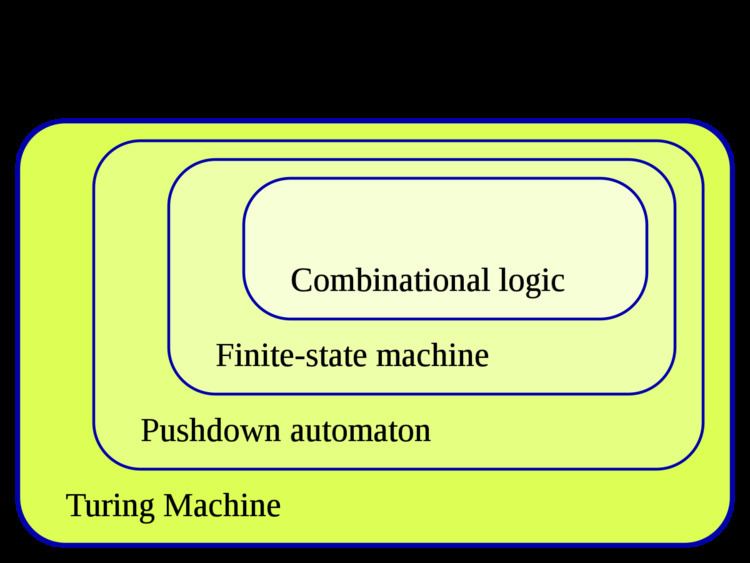
A Turing machine is equivalent to a pushdown automaton that has been made more flexible and concise by relaxing the last-in-first-out requirement of its stack.

At the other extreme, some very simple models turn out to be Turing-equivalent, i.e. to have the same computational power as the Turing machine model.

Common equivalent models are the multi-tape Turing machine, multi-track Turing machine, machines with input and output, and the non-deterministic Turing machine (NDTM) as opposed to the deterministic Turing machine (DTM) for which the action table has at most one entry for each combination of symbol and state.

Read-only, right-moving Turing machines are equivalent to NDFAs (as well as DFAs by conversion using the NDFA to DFA conversion algorithm).

For practical and didactical intentions the equivalent register machine can be used as a usual assembly programming language.

Choice c-machines, oracle o-machines

Early in his paper (1936) Turing makes a distinction between an "automatic machine"—its "motion ... completely determined by the configuration" and a "choice machine":

...whose motion is only partially determined by the configuration ... When such a machine reaches one of these ambiguous configurations, it cannot go on until some arbitrary choice has been made by an external operator. This would be the case if we were using machines to deal with axiomatic systems.

Turing (1936) does not elaborate further except in a footnote in which he describes how to use an a-machine to "find all the provable formulae of the [Hilbert] calculus" rather than use a choice machine. He "suppose[s] that the choices are always between two possibilities 0 and 1. Each proof will then be determined by a sequence of choices i₁, i₂, ..., i_n (i₁ = 0 or 1, i₂ = 0 or 1, ..., i_n = 0 or 1), and hence the number 2ⁿ + i₁2^n-1 + i₂2^n-2 + ... +i_n completely determines the proof. The automatic machine carries out successively proof 1, proof 2, proof 3, ..." (Footnote ‡, The Undecidable, p. 138)

This is indeed the technique by which a deterministic (i.e. a-) Turing machine can be used to mimic the action of a nondeterministic Turing machine; Turing solved the matter in a footnote and appears to dismiss it from further consideration.

An oracle machine or o-machine is a Turing a-machine that pauses its computation at state "o" while, to complete its calculation, it "awaits the decision" of "the oracle"—an unspecified entity "apart from saying that it cannot be a machine" (Turing (1939), The Undecidable, p. 166–168). The concept is now actively used by mathematicians.

Universal Turing machines

As Turing wrote in The Undecidable, p. 128 (italics added):

It is possible to invent a single machine which can be used to compute any computable sequence. If this machine U is supplied with the tape on the beginning of which is written the string of quintuples separated by semicolons of some computing machine M, then U will compute the same sequence as M.

This finding is now taken for granted, but at the time (1936) it was considered astonishing. The model of computation that Turing called his "universal machine"—"U" for short—is considered by some (cf. Davis (2000)) to have been the fundamental theoretical breakthrough that led to the notion of the stored-program computer.

Turing's paper ... contains, in essence, the invention of the modern computer and some of the programming techniques that accompanied it.

In terms of computational complexity, a multi-tape universal Turing machine need only be slower by logarithmic factor compared to the machines it simulates. This result was obtained in 1966 by F. C. Hennie and R. E. Stearns. (Arora and Barak, 2009, theorem 1.9)

Comparison with real machines

It is often said that Turing machines, unlike simpler automata, are as powerful as real machines, and are able to execute any operation that a real program can. What is neglected in this statement is that, because a real machine can only have a finite number of configurations, this "real machine" is really nothing but a linear bounded automaton. On the other hand, Turing machines are equivalent to machines that have an unlimited amount of storage space for their computations. However, Turing machines are not intended to model computers, but rather they are intended to model computation itself. Historically, computers, which compute only on their (fixed) internal storage, were developed only later.

There are a number of ways to explain why Turing machines are useful models of real computers:

1. Anything a real computer can compute, a Turing machine can also compute. For example: "A Turing machine can simulate any type of subroutine found in programming languages, including recursive procedures and any of the known parameter-passing mechanisms" (Hopcroft and Ullman p. 157). A large enough FSA can also model any real computer, disregarding IO. Thus, a statement about the limitations of Turing machines will also apply to real computers.
2. The difference lies only with the ability of a Turing machine to manipulate an unbounded amount of data. However, given a finite amount of time, a Turing machine (like a real machine) can only manipulate a finite amount of data.
3. Like a Turing machine, a real machine can have its storage space enlarged as needed, by acquiring more disks or other storage media. If the supply of these runs short, the Turing machine may become less useful as a model. But the fact is that neither Turing machines nor real machines need astronomical amounts of storage space in order to perform useful computation. The processing time required is usually much more of a problem.
4. Descriptions of real machine programs using simpler abstract models are often much more complex than descriptions using Turing machines. For example, a Turing machine describing an algorithm may have a few hundred states, while the equivalent deterministic finite automaton (DFA) on a given real machine has quadrillions. This makes the DFA representation infeasible to analyze.
5. Turing machines describe algorithms independent of how much memory they use. There is a limit to the memory possessed by any current machine, but this limit can rise arbitrarily in time. Turing machines allow us to make statements about algorithms which will (theoretically) hold forever, regardless of advances in conventional computing machine architecture.
6. Turing machines simplify the statement of algorithms. Algorithms running on Turing-equivalent abstract machines are usually more general than their counterparts running on real machines, because they have arbitrary-precision data types available and never have to deal with unexpected conditions (including, but not limited to, running out of memory).

One way in which Turing machines are a poor model for programs is that many real programs, such as operating systems and word processors, are written to receive unbounded input over time, and therefore do not halt. Turing machines do not model such ongoing computation well (but can still model portions of it, such as individual procedures).

Computational complexity theory

A limitation of Turing machines is that they do not model the strengths of a particular arrangement well. For instance, modern stored-program computers are actually instances of a more specific form of abstract machine known as the random access stored program machine or RASP machine model. Like the Universal Turing machine the RASP stores its "program" in "memory" external to its finite-state machine's "instructions". Unlike the universal Turing machine, the RASP has an infinite number of distinguishable, numbered but unbounded "registers"—memory "cells" that can contain any integer (cf. Elgot and Robinson (1964), Hartmanis (1971), and in particular Cook-Rechow (1973); references at random access machine). The RASP's finite-state machine is equipped with the capability for indirect addressing (e.g. the contents of one register can be used as an address to specify another register); thus the RASP's "program" can address any register in the register-sequence. The upshot of this distinction is that there are computational optimizations that can be performed based on the memory indices, which are not possible in a general Turing machine; thus when Turing machines are used as the basis for bounding running times, a 'false lower bound' can be proven on certain algorithms' running times (due to the false simplifying assumption of a Turing machine). An example of this is binary search, an algorithm that can be shown to perform more quickly when using the RASP model of computation rather than the Turing machine model.

Concurrency

Another limitation of Turing machines is that they do not model concurrency well. For example, there is a bound on the size of integer that can be computed by an always-halting nondeterministic Turing machine starting on a blank tape. (See article on unbounded nondeterminism.) By contrast, there are always-halting concurrent systems with no inputs that can compute an integer of unbounded size. (A process can be created with local storage that is initialized with a count of 0 that concurrently sends itself both a stop and a go message. When it receives a go message, it increments its count by 1 and sends itself a go message. When it receives a stop message, it stops with an unbounded number in its local storage.)

History

They were described in 1936 by Alan Turing.

Historical background: computational machinery

Robin Gandy (1919–1995)—a student of Alan Turing (1912–1954) and his lifelong friend—traces the lineage of the notion of "calculating machine" back to Babbage (circa 1834) and actually proposes "Babbage's Thesis":

That the whole of development and operations of analysis are now capable of being executed by machinery.

Gandy's analysis of Babbage's Analytical Engine describes the following five operations (cf. p. 52–53):

1. The arithmetic functions +, −, × where − indicates "proper" subtraction x − y = 0 if y ≥ x
2. Any sequence of operations is an operation
3. Iteration of an operation (repeating n times an operation P)
4. Conditional iteration (repeating n times an operation P conditional on the "success" of test T)
5. Conditional transfer (i.e. conditional "goto").

Gandy states that "the functions which can be calculated by (1), (2), and (4) are precisely those which are Turing computable." (p. 53). He cites other proposals for "universal calculating machines" including those of Percy Ludgate (1909), Leonardo Torres y Quevedo (1914), Maurice d'Ocagne (1922), Louis Couffignal (1933), Vannevar Bush (1936), Howard Aiken (1937). However:

... the emphasis is on programming a fixed iterable sequence of arithmetical operations. The fundamental importance of conditional iteration and conditional transfer for a general theory of calculating machines is not recognized ...

The Entscheidungsproblem (the "decision problem"): Hilbert's tenth question of 1900

With regard to Hilbert's problems posed by the famous mathematician David Hilbert in 1900, an aspect of problem #10 had been floating about for almost 30 years before it was framed precisely. Hilbert's original expression for #10 is as follows:

10. Determination of the solvability of a Diophantine equation. Given a Diophantine equation with any number of unknown quantities and with rational integral coefficients: To devise a process according to which it can be determined in a finite number of operations whether the equation is solvable in rational integers. The Entscheidungsproblem [decision problem for first-order logic] is solved when we know a procedure that allows for any given logical expression to decide by finitely many operations its validity or satisfiability ... The Entscheidungsproblem must be considered the main problem of mathematical logic.

By 1922, this notion of "Entscheidungsproblem" had developed a bit, and H. Behmann stated that

... most general form of the Entscheidungsproblem [is] as follows:

A quite definite generally applicable prescription is required which will allow one to decide in a finite number of steps the truth or falsity of a given purely logical assertion ...

Behmann remarks that ... the general problem is equivalent to the problem of deciding which mathematical propositions are true.

If one were able to solve the Entscheidungsproblem then one would have a "procedure for solving many (or even all) mathematical problems".

By the 1928 international congress of mathematicians, Hilbert "made his questions quite precise. First, was mathematics complete ... Second, was mathematics consistent ... And thirdly, was mathematics decidable?" (Hodges p. 91, Hawking p. 1121). The first two questions were answered in 1930 by Kurt Gödel at the very same meeting where Hilbert delivered his retirement speech (much to the chagrin of Hilbert); the third—the Entscheidungsproblem—had to wait until the mid-1930s.

The problem was that an answer first required a precise definition of "definite general applicable prescription", which Princeton professor Alonzo Church would come to call "effective calculability", and in 1928 no such definition existed. But over the next 6–7 years Emil Post developed his definition of a worker moving from room to room writing and erasing marks per a list of instructions (Post 1936), as did Church and his two students Stephen Kleene and J. B. Rosser by use of Church's lambda-calculus and Gödel's recursion theory (1934). Church's paper (published 15 April 1936) showed that the Entscheidungsproblem was indeed "undecidable" and beat Turing to the punch by almost a year (Turing's paper submitted 28 May 1936, published January 1937). In the meantime, Emil Post submitted a brief paper in the fall of 1936, so Turing at least had priority over Post. While Church refereed Turing's paper, Turing had time to study Church's paper and add an Appendix where he sketched a proof that Church's lambda-calculus and his machines would compute the same functions.

But what Church had done was something rather different, and in a certain sense weaker. ... the Turing construction was more direct, and provided an argument from first principles, closing the gap in Church's demonstration.

And Post had only proposed a definition of calculability and criticized Church's "definition", but had proved nothing.

Alan Turing's a-machine

In the spring of 1935, Turing as a young Master's student at King's College Cambridge, UK, took on the challenge; he had been stimulated by the lectures of the logician M. H. A. Newman "and learned from them of Gödel's work and the Entscheidungsproblem ... Newman used the word 'mechanical' ... In his obituary of Turing 1955 Newman writes:

To the question 'what is a "mechanical" process?' Turing returned the characteristic answer 'Something that can be done by a machine' and he embarked on the highly congenial task of analysing the general notion of a computing machine.

Gandy states that:

I suppose, but do not know, that Turing, right from the start of his work, had as his goal a proof of the undecidability of the Entscheidungsproblem. He told me that the 'main idea' of the paper came to him when he was lying in Grantchester meadows in the summer of 1935. The 'main idea' might have either been his analysis of computation or his realization that there was a universal machine, and so a diagonal argument to prove unsolvability.

While Gandy believed that Newman's statement above is "misleading", this opinion is not shared by all. Turing had a lifelong interest in machines: "Alan had dreamt of inventing typewriters as a boy; [his mother] Mrs. Turing had a typewriter; and he could well have begun by asking himself what was meant by calling a typewriter 'mechanical'" (Hodges p. 96). While at Princeton pursuing his PhD, Turing built a Boolean-logic multiplier (see below). His PhD thesis, titled "Systems of Logic Based on Ordinals", contains the following definition of "a computable function":

It was stated above that 'a function is effectively calculable if its values can be found by some purely mechanical process'. We may take this statement literally, understanding by a purely mechanical process one which could be carried out by a machine. It is possible to give a mathematical description, in a certain normal form, of the structures of these machines. The development of these ideas leads to the author's definition of a computable function, and to an identification of computability with effective calculability. It is not difficult, though somewhat laborious, to prove that these three definitions [the 3rd is the λ-calculus] are equivalent.

When Turing returned to the UK he ultimately became jointly responsible for breaking the German secret codes created by encryption machines called "The Enigma"; he also became involved in the design of the ACE (Automatic Computing Engine), "[Turing's] ACE proposal was effectively self-contained, and its roots lay not in the EDVAC [the USA's initiative], but in his own universal machine" (Hodges p. 318). Arguments still continue concerning the origin and nature of what has been named by Kleene (1952) Turing's Thesis. But what Turing did prove with his computational-machine model appears in his paper On Computable Numbers, With an Application to the Entscheidungsproblem (1937):

[that] the Hilbert Entscheidungsproblem can have no solution ... I propose, therefore to show that there can be no general process for determining whether a given formula U of the functional calculus K is provable, i.e. that there can be no machine which, supplied with any one U of these formulae, will eventually say whether U is provable.

Turing's example (his second proof): If one is to ask for a general procedure to tell us: "Does this machine ever print 0", the question is "undecidable".

1937–1970: The "digital computer", the birth of "computer science"

In 1937, while at Princeton working on his PhD thesis, Turing built a digital (Boolean-logic) multiplier from scratch, making his own electromechanical relays (Hodges p. 138). "Alan's task was to embody the logical design of a Turing machine in a network of relay-operated switches ..." (Hodges p. 138). While Turing might have been just initially curious and experimenting, quite-earnest work in the same direction was going in Germany (Konrad Zuse (1938)), and in the United States (Howard Aiken) and George Stibitz (1937); the fruits of their labors were used by the Axis and Allied military in World War II (cf. Hodges p. 298–299). In the early to mid-1950s Hao Wang and Marvin Minsky reduced the Turing machine to a simpler form (a precursor to the Post-Turing machine of Martin Davis); simultaneously European researchers were reducing the new-fangled electronic computer to a computer-like theoretical object equivalent to what was now being called a "Turing machine". In the late 1950s and early 1960s, the coincidentally parallel developments of Melzak and Lambek (1961), Minsky (1961), and Shepherdson and Sturgis (1961) carried the European work further and reduced the Turing machine to a more friendly, computer-like abstract model called the counter machine; Elgot and Robinson (1964), Hartmanis (1971), Cook and Reckhow (1973) carried this work even further with the register machine and random access machine models—but basically all are just multi-tape Turing machines with an arithmetic-like instruction set.

1970–present: the Turing machine as a model of computation

Today, the counter, register and random-access machines and their sire the Turing machine continue to be the models of choice for theorists investigating questions in the theory of computation. In particular, computational complexity theory makes use of the Turing machine:

Depending on the objects one likes to manipulate in the computations (numbers like nonnegative integers or alphanumeric strings), two models have obtained a dominant position in machine-based complexity theory:

the off-line multitape Turing machine..., which represents the standard model for string-oriented computation, and the random access machine (RAM) as introduced by Cook and Reckhow ..., which models the idealized Von Neumann style computer.

Only in the related area of analysis of algorithms this role is taken over by the RAM model.