Quantum stochastic calculus - Alchetron, the free social encyclopedia

Quantum stochastic calculus is a generalization of stochastic calculus to noncommuting variables. The tools provided by quantum stochastic calculus are of great use for modeling the random evolution of systems undergoing measurement, as in quantum trajectories. Just as the Lindblad master equation provides a quantum generalization to the Fokker-Planck equation, quantum stochastic calculus allows for the derivation of quantum stochastic differential equations (QSDE) that are analogous to classical Langevin equations.

Heat baths

An important physical scenario in which a quantum stochastic calculus is needed is the case of a system interacting with a heat bath. It is appropriate in many circumstances to model the heat bath as an assembly of harmonic oscillators. One type of interaction between the system and the bath can be modeled (after making a canonical transformation) by the following Hamiltonian:

H = H s y s ( Z ) + 1 2 ∑ n ( ( p n − κ n X ) 2 + ω n 2 q n 2 ) ,

where H s y s is the system Hamiltonian, Z is a vector containing the system variables corresponding to a finite number of degrees of freedom, n is an index for the different bath modes, ω n is the frequency of a particular mode, p n and q n are bath operators for a particular mode, X is a system operator, and κ n quantifies the coupling between the system and a particular bath mode.

In this scenario the equation of motion for an arbitrary system operator Y is called the quantum Langevin equation and may be written as:

where [ ⋅ , ⋅ ] and { ⋅ , ⋅ } denote the commutator and anticommutator (respectively), the memory function f is defined as:

f ( t ) ≡ ∑ n κ n 2 cos ⁡ ( ω n t ) ,

and the time dependent noise operator ξ is defined as:

ξ ( t ) ≡ i ∑ n κ n ℏ ω n 2 ( − a n ( t 0 ) e − i ω n ( t − t 0 ) + a n † ( t 0 ) e i ω n ( t − t 0 ) ) ,

where the bath annihilation operator a n is defined as:

a n ≡ ω n q n + i p n 2 ℏ ω n .

Oftentimes this equation is more general than is needed, and further approximations are made to simplify the equation.

White noise formalism

For many purposes it is convenient to make approximations about the nature of the heat bath in order to achieve a white noise formalism. In such a case the interaction may be modeled by the Hamiltonian H = H s y s + H B + H i n t where:

H B = ℏ ∫ − ∞ ∞ d ω ω b † ( ω ) b ( ω ) ,

and

H i n t = i ℏ ∫ − ∞ ∞ d ω κ ( ω ) ( b † ( ω ) c − c † b ( ω ) ) ,

where b ( ω ) are annihilation operators for the bath with the commutation relation [ b ( ω ) , b † ( ω ′ ) ] = δ ( ω − ω ′ ) , c is an operator on the system, κ ( ω ) quantifies the strength of the coupling of the bath modes to the system, and H s y s describes the free system evolution. This model uses the rotating wave approximation and extends the lower limit of ω to − ∞ in order to admit a mathematically simple white noise formalism. The coupling strengths are also usually simplified to a constant in what is sometimes called the first Markov approximation:

κ ( ω ) = γ 2 π .

Systems coupled to a bath of harmonic oscillators can be thought of as being driven by a noise input and radiating a noise output. The input noise operator at time t is defined by:

b i n ( t ) = 1 2 π ∫ − ∞ ∞ d ω e − i ω ( t − t 0 ) b 0 ( ω ) ,

where b 0 ( ω ) = b ( ω ) | t = t 0 , since this operator is expressed in the Heisenberg picture. Satisfaction of the commutation relation [ b i n ( t ) , b i n † ( t ′ ) ] = δ ( t − t ′ ) allows the model to have a strict correspondence with a Markovian master equation.

In the white noise setting described so far, the quantum Langevin equation for an arbitrary system operator a takes a simpler form:

For the case most closely corresponding to classical white noise, the input to the system is described by a density operator giving the following expectation value:

Quantum Wiener process

In order to define quantum stochastic integration, it is important to define a quantum Wiener process:

B ( t , t 0 ) = ∫ t 0 t b i n ( t ′ ) d t ′ .

This definition gives the quantum Wiener process the commutation relation [ B ( t , t 0 ) , B † ( t , t 0 ) ] = t − t 0 . The property of the bath annihilation operators in (WN2) implies that the quantum Wiener process has an expectation value of:

⟨ B † ( t , t 0 ) B ( t , t 0 ) ⟩ ρ ( t , t 0 ) = N ( t − t 0 ) .

The quantum Wiener processes are also specified such that their quasiprobability distributions are Gaussian by defining the density operator:

ρ ( t , t 0 ) = ( 1 − e − κ ) exp ⁡ [ − κ B † ( t , t 0 ) B ( t , t 0 ) t − t 0 ] ,

where N = 1 / ( e κ − 1 ) .

Quantum stochastic integration

The stochastic evolution of system operators can also be defined in terms of the stochastic integration of given equations.

Quantum Itō integral

The quantum Itō integral of a system operator g ( t ) is given by:

( I ) ∫ t 0 t g ( t ′ ) d B ( t ′ ) = lim n → ∞ ∑ i = 1 n g ( t i ) ( B ( t i + 1 , t 0 ) − B ( t i , t 0 ) ) ,

where the bold (I) preceding the integral stands for Itō. One of the characteristics of defining the integral in this way is that the increments d B and d B † commute with the system operator.

Itō quantum stochastic differential equation

In order to define the Itō QSDE, it is necessary to know something about the bath statistics. In the context of the white noise formalism described earlier, the Itō QSDE can be defined as:

( I ) d a = − i ℏ [ a , H s y s ] d t + γ ( ( N + 1 ) D [ c † ] a + N D [ c ] a ) d t − γ ( [ a , c † ] d B ( t ) − d B † ( t ) [ a , c ] ) ,

where the equation has been simplified using the Lindblad superoperator:

D [ A ] a ≡ A a A † − 1 2 ( A † A a + a A † A ) .

This differential equation is interpreted as defining the system operator a as the quantum Itō integral of the right hand side, and is equivalent to the Langevin equation (WN1).

Quantum Stratonovich integral

The quantum Stratonovich integral of a system operator g ( t ) is given by:

( S ) ∫ t 0 t g ( t ′ ) d B ( t ′ ) = lim n → ∞ ∑ i = 1 n g ( t i ) + g ( t i + 1 ) 2 ( B ( t i + 1 , t 0 ) − B ( t i , t 0 ) ) ,

where the bold (S) preceding the integral stands for Stratonovich. Unlike the Itō formulation, the increments in the Stratonovich integral do not commute with the system operator, and it can be shown that:

( S ) ∫ t 0 t g ( t ′ ) d B ( t ′ ) − ( S ) ∫ t 0 t d B ( t ′ ) g ( t ′ ) = γ 2 ∫ t 0 t d t ′ [ g ( t ′ ) , c ( t ′ ) ] .

Stratonovich quantum stochastic differential equation

The Stratonovich QSDE can be defined as:

( S ) d a = − i ℏ [ a , H s y s ] d t − γ 2 ( [ a , c † ] c − c † [ a , c ] ) d t − γ ( [ a , c † ] d B ( t ) − d B † ( t ) [ a , c ] ) .

This differential equation is interpreted as defining the system operator a as the quantum Stratonovich integral of the right hand side, and is in the same form as the Langevin equation (WN1).

Relation between Itō and Stratonovich integrals

The two definitions of quantum stochastic integrals relate to one another in the following way, assuming a bath with N defined as before:

( S ) ∫ t 0 t g ( t ′ ) d B ( t ′ ) = ( I ) ∫ t 0 t g ( t ′ ) d B ( t ′ ) + 1 2 γ N ∫ t 0 t d t ′ [ g ( t ′ ) , c ( t ′ ) ] .

Calculus rules

Just as with classical stochastic calculus, the appropriate product rule can be derived for Itō and Stratonovich integration, respectively:

( I ) d ( a b ) = a d b + b d a + d a d b , ( S ) d ( a b ) = a d b + d a b .

As is the case in classical stochastic calculus, the Stratonovich form is the one which preserves the ordinary calculus (which in this case is noncommuting). A peculiarity in the quantum generalization is the necessity to define both Itō and Stratonovitch integration in order to prove that the Stratonovitch form preserves the rules of noncommuting calculus.

Quantum trajectories

Quantum trajectories can generally be thought of as the path through Hilbert space that the state of a quantum system traverses over time. In a stochastic setting, these trajectories are often conditioned upon measurement results. The unconditioned Markovian evolution of a quantum system (averaged over all possible measurement outcomes) is given by a Lindblad equation. In order to describe the conditioned evolution in these cases, it is necessary to unravel the Lindblad equation by choosing a consistent QSDE. In the case where the conditioned system state is always pure, the unraveling could be in the form of a stochastic Schrödinger equation (SSE). If the state may become mixed, then it is necessary to use a stochastic master equation (SME).

Example unravelings

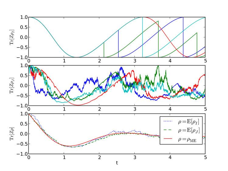
Consider the following Lindblad master equation for a system interacting with a vacuum bath:

ρ ˙ = D [ c ] ρ − i [ H s y s , ρ ] .

This describes the evolution of the system state averaged over the outcomes of any particular measurement that might be made on the bath. The following SME describes the evolution of the system conditioned on the results of a continuous photon-counting measurement performed on the bath:

d ρ I ( t ) = ( d N ( t ) G [ c ] − d t H [ i H s y s + 1 2 c † c ] ) ρ I ( t ) ,

where

G [ r ] ρ ≡ r ρ r † Tr ⁡ [ r ρ r † ] − ρ H [ r ] ρ ≡ r ρ + ρ r † − Tr ⁡ [ r ρ + ρ r † ] ρ

are nonlinear superoperators and N ( t ) is the photocount, indicating how many photons have been detected at time t and giving the following jump probability:

E ⁡ [ d N ( t ) ] = d t Tr ⁡ [ c † c ρ I ( t ) ] ,

where E ⁡ [ ⋅ ] denotes the expected value. Another type of measurement that could be made on the bath is homodyne detection, which results in quantum trajectories given by the following SME:

d ρ J ( t ) = − i [ H s y s , ρ J ( t ) ] d t + d t D [ c ] ρ J ( t ) + d W ( t ) H [ c ] ρ J ( t ) ,

where d W ( t ) is a Wiener increment satisfying:

d W ( t ) 2 = d t E ⁡ [ d W ( t ) ] = 0 .

Although these two SMEs look wildly different, calculating their expected evolution shows that they are both indeed unravelings of the same Lindlad master equation:

E ⁡ [ d ρ I ( t ) ] = E ⁡ [ d ρ J ( t ) ] = ρ ˙ d t .

Computational considerations

One important application of quantum trajectories is reducing the computational resources required to simulate a master equation. For a Hilbert space of dimension d, the amount of real numbers required to store the density matrix is of order d², and the time required to compute the master equation evolution is of order d⁴. Storing the state vector for a SSE, on the other hand, only requires an amount of real numbers of order d, and the time to compute trajectory evolution is only of order d². The master equation evolution can then be approximated by averaging over many individual trajectories simulated using the SSE, a technique sometimes referred to as the Monte Carlo wave-function approach. Although the number of calculated trajectories n must be very large in order to accurately approximate the master equation, good results can be obtained for trajectory counts much less than d². Not only does this technique yield faster computation time, but it also allows for the simulation of master equations on machines that do not have enough memory to store the entire density matrix.

References

Quantum stochastic calculus Wikipedia

(Text) CC BY-SA

Contents